ABSTRACT (original thesis): Studying the geometry of sets appearing in various problems of quantum information helps in understanding different parts of the theory. It is thus worthwhile to approach quantum mechanics from the angle of geometry – this has already provided a multitude of interesting results. In this thesis I demonstrate results relevant to numerical ranges – the sets of simultaneously attainable expectation values of several observables. In particular, I apply this notion in the problems related to uncertainty relations, entanglement detection, and determining bounds for the value of spectral gap. Apart from this, I present geometric structures helping with the question of state interconversion using channels commuting with a particular representation of a group. CITATION (original thesis): Konrad Szymański (2023), Numerical ranges and geometry in quantum information: Entanglement, uncertainty relations, phase transitions, and state interconversion. arXiv:2303.07390. https://doi.org/10.48550/arXiv.2303.07390. CITATION (original article): Konrad Szymański, Stephan Weis, Karol Życzkowski, Classification of joint numerical ranges of three hermitian matrices of size three, Linear Algebra and its Applications, 545, 148-173. https://doi.org/10.1016/j.laa.2017.11.017
Quantum information: quantum mechanics in finite dimensions
Quantum information: quantum mechanics in finite dimensions
In introductory quantum mechanics lectures the state of a system is represented by a wavefunction, describing probability amplitudes in every point of space. A classic toy example (which is still a relevant model for e.g. quantum state of light) is a one-dimensional harmonic oscillator, where the dynamics is governed by the Schrödinger equation
ihψ(x,t)=ψ(x,t)
∂
∂t
-+
2
h
2m
2
∂
x
m
2
ω
2
x
2
H
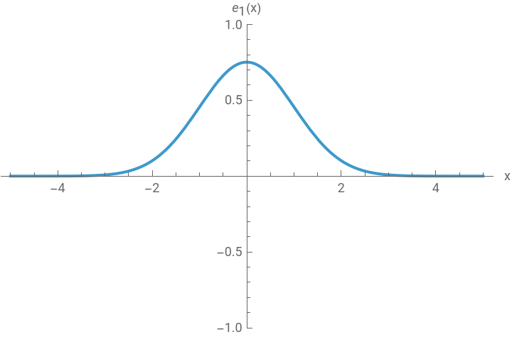
One of the standard methods of solving this equation for given initial function (a function ) is to find the eigensystem of the differential operator – the Hamiltonian. These are the functions (x) (with appropriate regularity constraints) such that for some real number , called the energy of the state described by (x). All reasonable wavefunctions can be expressed as (potentially infinite) sums of the eigenfunctions .
Let’s see how they look like for the harmonic oscillator! First, let’s calculate some of them:
ψ(x,t=0)
H
e
n
H(x)=(x)
e
n
E
n
e
n
E
n
e
n
{}
e
n
Let’s see how they look like for the harmonic oscillator! First, let’s calculate some of them:
In[]:=
schroedinger=D[ψ[x],{x,2}]+mψ[x];$Assumptions={ℏ>0,m>0,ω>0,x∈Reals,t∈Reals};nstates=10;eigensystem=DEigensystem[schroedinger,ψ[x],{x,-∞,∞},nstates,Method->"Normalize"]
-
2
ℏ
2m
1
2
2
ω
2
x
Out[]=
,,,x,,-2+,,-12x+8,,12+-,,120x-160+32,,-120+-+,,-1680x+3360-1344+128,,1680+-+-,,30240x-80640+48384-9216+512
ωℏ
2
-
mω
2
x
2ℏ
1/4
(mωℏ)
1/4
π
ℏ
3ωℏ
2
2
-
mω
2
x
2ℏ
3/4
mω
ℏ
1/4
π
5ωℏ
2
-
mω
2
x
2ℏ
4mω
2
x
ℏ
1/4
(mωℏ)
2
2
1/4
π
ℏ
7ωℏ
2
-
mω
2
x
2ℏ
mω
ℏ
3
x
3/2
mω
ℏ
1/4
(mωℏ)
4
3
1/4
π
ℏ
9ωℏ
2
-
mω
2
x
2ℏ
16
2
m
4
x
2
ω
2
ℏ
48mω
2
x
ℏ
1/4
(mωℏ)
8
6
1/4
π
ℏ
11ωℏ
2
-
mω
2
x
2ℏ
mω
ℏ
3
x
3/2
mω
ℏ
5
x
5/2
mω
ℏ
1/4
(mωℏ)
16
15
1/4
π
ℏ
13ωℏ
2
-
mω
2
x
2ℏ
64
3
m
6
x
3
ω
3
ℏ
480
2
m
4
x
2
ω
2
ℏ
720mω
2
x
ℏ
1/4
mω
ℏ
96
5
1/4
π
15ωℏ
2
-
mω
2
x
2ℏ
mω
ℏ
3
x
3/2
mω
ℏ
5
x
5/2
mω
ℏ
7
x
7/2
mω
ℏ
1/4
(mωℏ)
96
70
1/4
π
ℏ
17ωℏ
2
-
mω
2
x
2ℏ
256
4
m
8
x
4
ω
4
ℏ
3584
3
m
6
x
3
ω
3
ℏ
13440
2
m
4
x
2
ω
2
ℏ
13440mω
2
x
ℏ
1/4
mω
ℏ
384
70
1/4
π
19ωℏ
2
-
mω
2
x
2ℏ
mω
ℏ
3
x
3/2
mω
ℏ
5
x
5/2
mω
ℏ
7
x
7/2
mω
ℏ
9
x
9/2
mω
ℏ
1/4
(mωℏ)
2304
35
1/4
π
ℏ
Physical systems have a lower bound to the available energy – hence, we can expect that a state of lowest possible energy could exist. Indeed it does, and it is called the ground state of the Hamiltonian . For a simple harmonic oscillator, the states are discrete and can be enumerated.
(evaluate the next cell for a plot)
H
(evaluate the next cell for a plot)
In[]:=
numvalues={ℏ->1,m->1,ω->1};ManipulatePlot,{n,1,nstates,1}
Out[]=


If a state can be initially written as , its subsequent evolution can be predicted. Since and , it can be inferred that each of the (x) terms is advanced by a phase factor and thus . Here we can expand an initial state in a finite subset of the entire basis (it is an approximation, but it works well enough) and the end state at arbitrary time can be written. The result can be used to visualize the state evolution. (evaluate the next cell for a plot)
ψ(x,t=0)= (x)
∑
n
c
n
e
n
H(x)=(x)
e
n
E
n
e
n
ihψ(x,t)=Hψ(x,t)
∂
t
e
n
ψ(x,t)=exp(-it)(x)
∑
n
c
n
E
n
e
n
t
In[]:=
numeigensystem=eigensystem/.numvalues;initstate=/.{x->2(x-1)};decomp={#1,#2,Integrate[#2initstate,{x,-∞,∞}]}&@@@numeigensystem;endstate=Total[({energy,eigenstate,prefactor}Exp[-energyt]prefactoreigenstate)@@@decomp]Manipulate[AbsArgPlot[#,{x,-3,3},PlotRange->{All,{-2,2}},AxesLabel->{"x (a.u.)","ψ(x,t)"}],{t,0,10}]&@endstate
2
-
2
x
2
1/4
π
Out[]=
2
---
2
5
t
2
2
x
2
5
1/4
π
16x
---
2
5
3t
2
2
x
2
5
5
1/4
π
17(-2+4)
---
2
5
5t
2
2
x
2
2
x
50
5
1/4
π
26(-12x+8)
---
2
5
7t
2
2
x
2
3
x
375
5
1/4
π
1181(12-48+16)
---
2
5
9t
2
2
x
2
2
x
4
x
30000
5
1/4
π
401(120x-160+32)
---
2
5
11t
2
2
x
2
3
x
5
x
187500
5
1/4
π
75743(-120+720-480+64)
---
2
5
13t
2
2
x
2
2
x
4
x
6
x
45000000
5
1/4
π
111833(-1680x+3360-1344+128)
---
2
5
15t
2
2
x
2
3
x
5
x
7
x
393750000
5
1/4
π
4374359(1680-13440+13440-3584+256)
---
2
5
17t
2
2
x
2
2
x
4
x
6
x
8
x
126000000000
5
1/4
π
17794319(30240x-80640+48384-9216+512)
---
2
5
19t
2
2
x
2
3
x
5
x
7
x
9
x
1417500000000
5
1/4
π
Out[]=
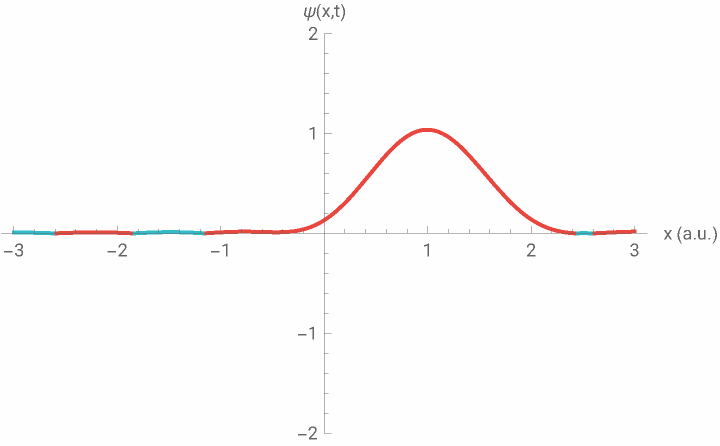
Remember that the wavefunction ψ(x,t) is complex: it carries the information about the probability of finding an object at certain point of space, but also the information about the momentum distribution and much more. For reasons still not entirely understood the probability density is related to the wavefunction via the Born rule: probability ∝ | amplitude . One could, for instance, calculate the probability of finding an object in the positive half-axis at :
2
|
(x>0)
t=1
In[]:=
probofpositive[τ_]:=NIntegrate[,{x,0,∞}]probofpositive[1]
2
Abs[endstate/.t->τ]
Out[]=
0.67332
… or plot the evolution as a function of time:
In[]:=
Plot[probofpositive[t],{t,0,10},AxesLabel->{"t (a.u.)","Probability"}]
Out[]=
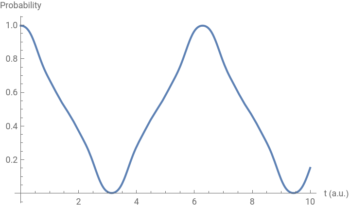
The probability as described above can be described by the use of concept of observable: an operator on the space of functions. The expectation value of an observable is then an inner product of ψ(x,t) with Ο ψ(x,t):
Ο
Ο
〈Ο〉
ψ
in mathematical and physical notation, respectively. For this particular case, the operator acts like Ο, where Θ(x) is the step function , so that the end expression is the integral
ψ(x,t)=Θ(x)ψ(x)
(Θ(x>=0)=1,Θ(x<0)=0)
〈Ο〉
ψ
*
ψ(x,t)
But this is not the only approach: the operator can also be expressed in the basis we are already working with, the eigenbasis of Hamiltonian . Let’s do it numerically! The result, constrained to the finite subset of the entire basis, is a square Hermitian matrix (in this case even real symmetric), with the matrix elements being the inner product of (x) and (x) :
Ο
H
e
n
Ο
e
n
In[]:=
Omatrix=(*〈|O|〉=*)Table[NIntegrate[v1v2,{x,0,∞},AccuracyGoal->10]//Chop,{v1,Last/@numeigensystem},{v2,Last/@numeigensystem}]//Chop;Omatrix//MatrixForm
e
n
e
m
Out[]//MatrixForm=
0.5 | 0.398942 | 0 | -0.162868 | 0 | 0.109255 | 0 | -0.0842919 | 0 | 0.0695373 |
0.398942 | 0.5 | 0.282095 | 0 | -0.0814338 | 0 | 0.0446031 | 0 | -0.0298017 | 0 |
0 | 0.282095 | 0.5 | 0.345494 | 0 | -0.128758 | 0 | 0.0834448 | 0 | -0.063219 |
-0.162868 | 0 | 0.345494 | 0.5 | 0.299207 | 0 | -0.0910457 | 0 | 0.0510993 | 0 |
0 | -0.0814338 | 0 | 0.299207 | 0.5 | 0.334523 | 0 | -0.120442 | 0 | 0.0766489 |
0.109255 | 0 | -0.128758 | 0 | 0.334523 | 0.5 | 0.305377 | 0 | -0.0952179 | 0 |
0 | 0.0446031 | 0 | -0.0910457 | 0 | 0.305377 | 0.5 | 0.329844 | 0 | -0.116618 |
-0.0842919 | 0 | 0.0834448 | 0 | -0.120442 | 0 | 0.329844 | 0.5 | 0.308541 | 0 |
0 | -0.0298017 | 0 | 0.0510993 | 0 | -0.0952179 | 0 | 0.308541 | 0.5 | 0.327257 |
0.0695373 | 0 | -0.063219 | 0 | 0.0766489 | 0 | -0.116618 | 0 | 0.327257 | 0.5 |
Let’s define the function to calculate the expectation values. Sometimes the state vectors may require normalization, hence the following form:
Let’s define the function to calculate the expectation values. Sometimes the state vectors may require normalization, hence the following form:
Note that this function only works for finite-dimensional vectors, which in Wolfram Language are described by lists of complex numbers. This description of course does not exactly capture the reality, but it is an important simplification of which a large part of quantum information relies on.
A qubit is exactly this: a two-dimensional simplification of a more complicated system. The two-dimensional subspaces forming a qubit vary between physical implementations (this could be different electronic levels of an atom or ion, subspace of only one photon in two polarization modes, or states of a quantized supercurrent). Full description is often too complex, requiring tools of functional analysis, and there is still plenty to learn from finite-dimensional systems.
A qubit is exactly this: a two-dimensional simplification of a more complicated system. The two-dimensional subspaces forming a qubit vary between physical implementations (this could be different electronic levels of an atom or ion, subspace of only one photon in two polarization modes, or states of a quantized supercurrent). Full description is often too complex, requiring tools of functional analysis, and there is still plenty to learn from finite-dimensional systems.
Probabilistic mixtures of state vectors and convex geometry
Probabilistic mixtures of state vectors and convex geometry
The three expectation values will then have the form of
There of course exist superpositions which could approximate the expectation value of a single operator. But they will always fail on others:
Ensembles define density operators, hence it is no surprise that the expectation values provided by both coincide:
Unfortunately, while the state space for a qubit is a simple 3D ball, this does not generalize. Even for a qutrit the relevant set of valid parameters is a nontrivial 8-dimensional convex set.
The reason behind this complexity is the fact that the boundary is defined by polynomial equations. The boundary of the qubit states is exactly the unit trace Hermitian matrices with vanishing determinant:
The reason behind this complexity is the fact that the boundary is defined by polynomial equations. The boundary of the qubit states is exactly the unit trace Hermitian matrices with vanishing determinant:
This is because for a boundary state, one of their eigenvalues has to vanish and so does the determinant. But the determinant polynomial becomes increasingly more complex with more variables as dimension grows.
In the next section we’ll study a simpler problem: the geometry of low-dimensional projections.
In the next section we’ll study a simpler problem: the geometry of low-dimensional projections.
Projections and intersections of the set of states: numerical ranges and spectrahedra
Projections and intersections of the set of states: numerical ranges and spectrahedra
Let’s try with a simple example first: two observables (here: matrices of size three), and just as a first approach let’s sample from the set of state vectors to obtain random tuples expectation values. With enough sample points, a shape starts to emerge.
(evaluate the next cell for a plot)
(evaluate the next cell for a plot)
But the result of the second optimization is known by reasoning similar to the one in the previous paragraphs: it is the maximal eigenvalue,
We have observed mathematical properties of joint numerical ranges, and learned how to obtain different descriptions of their geometry. In the next section they will be put to use.
Uncertainty relations can be found via polynomial theory
Uncertainty relations can be found via polynomial theory
The polynomial description of the boundary exists and can be calculated like in the previous section:
Then we need to ensure that the λ is an extremum. Everything here is analytical, therefore we can simply request that the derivative of the determinant vanishes, and get a final set of polynomial equations:
Then we need to solve this set of polynomial equations! Just as previously, we’ll use the systematic variable elimination provided by Gröbner bases to obtain a single polynomial in λ– the paraboloid shift – and find its minimal real solution. And the minimal real root coincides with the numerical result.
Conclusion
Conclusion
In this notebook we have defined the (joint) numerical range as the set of allowed expectation values for fixed observables:
Numerical ranges, under certain conditions, have convex dual descriptions by spectrahedra, affine subset of the set of positive semidefinite matrices:
Through polynomial description of the latter objects, strict results of problems in quantum information can be obtained. Still, there are multiple open problems (see the PhD thesis in reference 1). For instance:
References
References
1
.K.S., Numerical ranges and geometry in quantum information. Ph.D. thesis (arXiv: 2303.07390), 2022.
2
.K.S., S. Weis, K Życzkowski, Classification of joint numerical ranges of three Hermitian matrices of size three, LAA, 2018 (classification of numerical ranges geometry)
3
.J. Xie, et al. Observing geometry of quantum states in a three-level system. PRL, 2020.
(physical realization of the classification for three operators of size three in ref. 2)
(physical realization of the classification for three operators of size three in ref. 2)
4
.P. Giorda, L. Maccone, and A. Riccardi. State-independent uncertainty relations from eigenvalue minimization. PRA, 2019.
(connection between uncertainty relations and separable numerical ranges)
(connection between uncertainty relations and separable numerical ranges)
5
.D. Plaumann, R. Sinn, and S. Weis. Kippenhahn’s theorem for joint numerical ranges and quantum states. SIAGA, 2021.
(polynomial description of the boundary of numerical range)
(polynomial description of the boundary of numerical range)
CITE THIS NOTEBOOK
CITE THIS NOTEBOOK
Numerical ranges and geometry in quantum information
by Konrad Szymański
Wolfram Community, STAFF PICKS, April 4, 2024
https://community.wolfram.com/groups/-/m/t/3156048
by Konrad Szymański
Wolfram Community, STAFF PICKS, April 4, 2024
https://community.wolfram.com/groups/-/m/t/3156048