Digitizing and Plotting Nikuradse’s Turbulent Pipe Flow Data in Mathematica
Authors: Housam Binous and Ahmed Bellagi
Digitizing and Plotting Nikuradse’s Turbulent Pipe Flow Data in Mathematica
Authors: Housam Binous and Ahmed Bellagi
Authors: Housam Binous and Ahmed Bellagi
The experiments of Johann Nikuradse were conducted in the 1930s to study friction losses in turbulent pipe flow. Nikuradse used pipes whose inner walls were coated with uniform sand grains of known size, creating controlled roughness. By measuring the pressure drop for different flow velocities and roughness heights, he investigated how the friction factor depends on: (1) the Reynolds number (Re) and (2) the relative roughness.
His experiments showed three important flow regimes for turbulent flow:
1. Hydraulically smooth regime: Roughness has little effect; friction mainly depends on Reynolds number.
2. Transition regime: Both Reynolds number and wall roughness influence the friction factor.
3. Fully rough regime: Friction factor becomes independent of Reynolds number and depends only on relative roughness.
These experimental observation became fundamental for pipe-flow engineering and led to the development of the Moody chart and correlations such as the Colebrook-White equation.
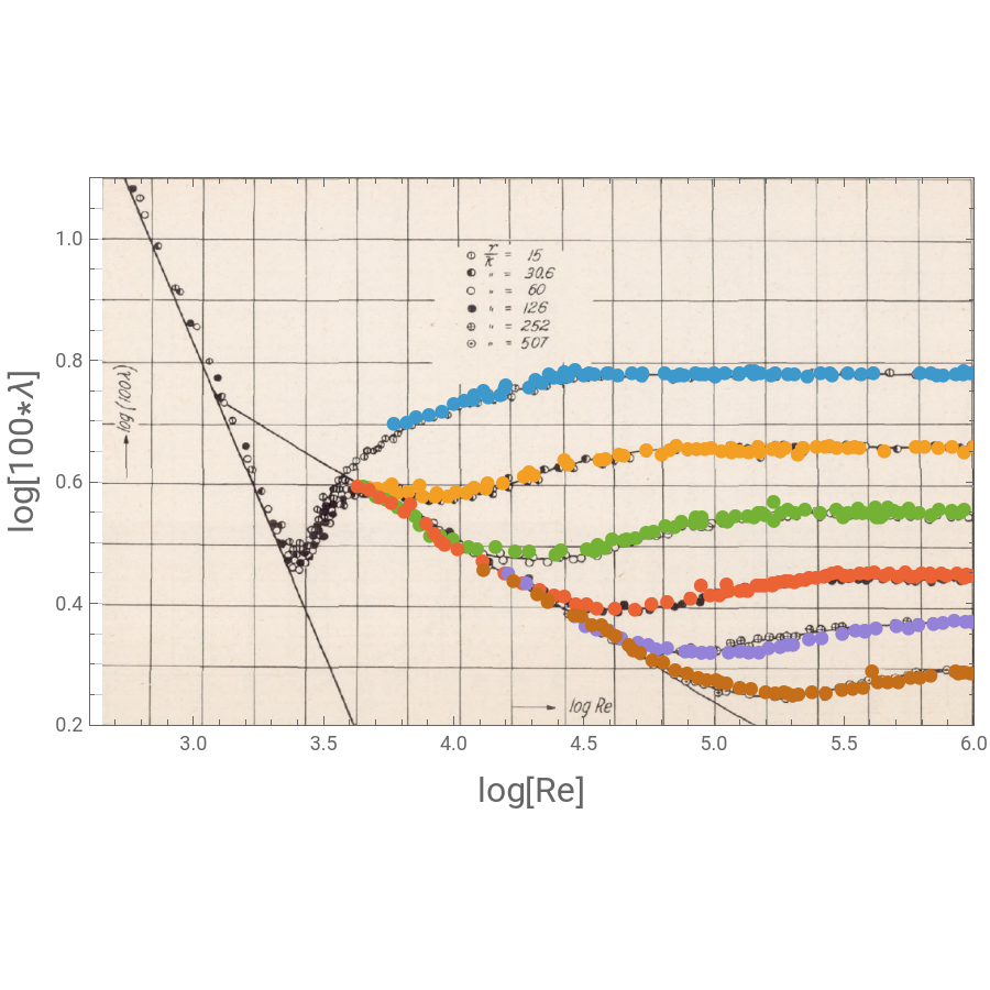
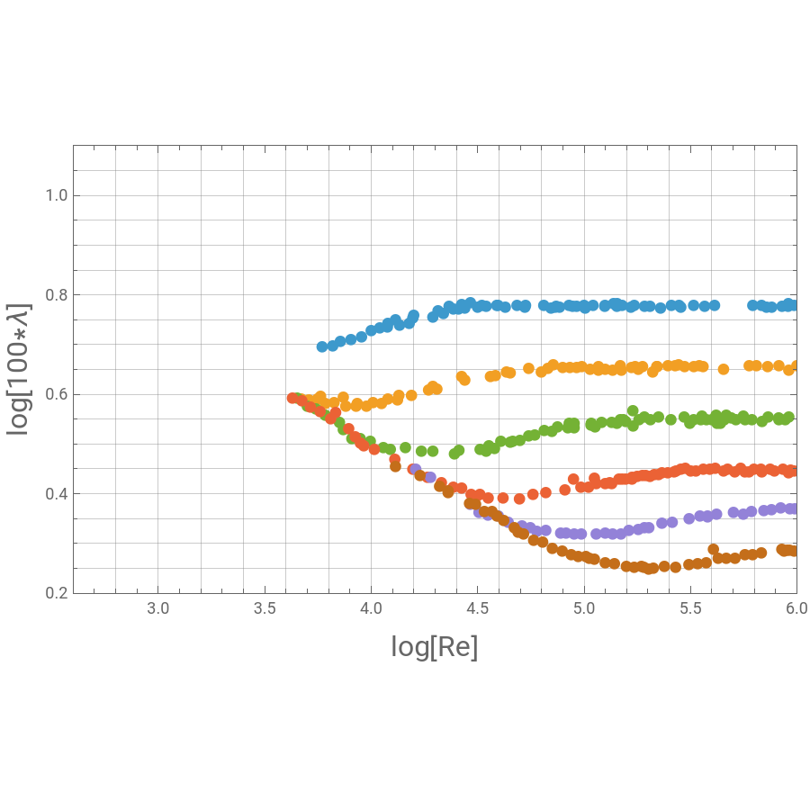
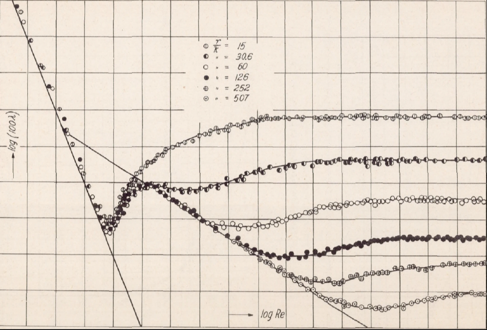
Here, we plot the classical experimental data of Nikuradse for turbulent flow in rough pipes (see Refs. 1-2). This plot represents the friction factor parameter ((100×λ)) as a function of the Reynolds number ( (Re) ) for several values of relative roughness ( ).
This plot allows readers to clearly visualize the different hydraulic flow regimes observed experimentally: the laminar regime, the transition region, and the fully turbulent rough regime. By digitizing and plotting the original data in Mathematica, the behavior of the friction factor becomes easier to analyze quantitatively and compare with empirical correlations such as the Haaland equation or the Colebrook-White equation.
The use of Mathematica also improves reproducibility and readability. Readers can directly inspect trends, validate numerical models, test fitting procedures, and study how roughness influences turbulent flow behavior across a wide Reynolds number range. This visualization is useful in fluid mechanics and chemical engineering. Indeed, it applies historical experimental results with modern technical computing environment such as Mathematica.
References:
[1] J. Nikuradse, “Strömungsgesetze in Rauhen Rohren,” VDI Forschungsh. 361, 1933.
[2] J. Nikuradze, Laws of flow in rough pipes, National Advisory Committee for Aeronautics, Washington, 1950.
His experiments showed three important flow regimes for turbulent flow:
1. Hydraulically smooth regime: Roughness has little effect; friction mainly depends on Reynolds number.
2. Transition regime: Both Reynolds number and wall roughness influence the friction factor.
3. Fully rough regime: Friction factor becomes independent of Reynolds number and depends only on relative roughness.
These experimental observation became fundamental for pipe-flow engineering and led to the development of the Moody chart and correlations such as the Colebrook-White equation.
Here, we plot the classical experimental data of Nikuradse for turbulent flow in rough pipes (see Refs. 1-2). This plot represents the friction factor parameter (
log
10
log
10
r/k
This plot allows readers to clearly visualize the different hydraulic flow regimes observed experimentally: the laminar regime, the transition region, and the fully turbulent rough regime. By digitizing and plotting the original data in Mathematica, the behavior of the friction factor becomes easier to analyze quantitatively and compare with empirical correlations such as the Haaland equation or the Colebrook-White equation.
The use of Mathematica also improves reproducibility and readability. Readers can directly inspect trends, validate numerical models, test fitting procedures, and study how roughness influences turbulent flow behavior across a wide Reynolds number range. This visualization is useful in fluid mechanics and chemical engineering. Indeed, it applies historical experimental results with modern technical computing environment such as Mathematica.
References:
[1] J. Nikuradse, “Strömungsgesetze in Rauhen Rohren,” VDI Forschungsh. 361, 1933.
[2] J. Nikuradze, Laws of flow in rough pipes, National Advisory Committee for Aeronautics, Washington, 1950.
In[]:=
data2={{4.114,0.456},{4.23,0.438},{4.322,0.417},{4.362,0.407},{4.362,0.403},{4.462,0.381},{4.491,0.38},{4.532,0.366},{4.568,0.365},{4.591,0.356},{4.623,0.347},{4.672,0.333},{4.69,0.324},{4.716,0.32},{4.763,0.307},{4.806,0.303},{4.851,0.292},{4.898,0.286},{4.94,0.278},{4.973,0.274},{5.009,0.274},{5.025,0.272},{5.049,0.27},{5.1,0.262},{5.143,0.26},{5.199,0.255},{5.236,0.253},{5.27,0.255},{5.281,0.253},{5.303,0.25},{5.326,0.252},{5.377,0.255},{5.43,0.253},{5.493,0.258},{5.534,0.26},{5.574,0.262},{5.608,0.29},{5.63,0.272},{5.668,0.272},{5.709,0.272},{5.756,0.278},{5.792,0.279},{5.833,0.283},{5.94,0.286},{5.965,0.288},{5.929,0.289},{5.954,0.288},{5.987,0.286}};
In[]:=
data3={{4.21,0.4506},{4.279,0.4349},{4.465,0.3808},{4.507,0.3636},{4.549,0.3579},{4.597,0.3562},{4.644,0.3434},{4.778,0.3257},{4.82,0.3282},{4.916,0.3222},{4.987,0.3197},{5.057,0.321},{5.1,0.3228},{5.173,0.3197},{5.21,0.3276},{5.283,0.3322},{5.366,0.3416},{5.494,0.3504},{5.58,0.3562},{5.623,0.3602},{5.702,0.3636},{4.708,0.3371},{5.305,0.3328},{5.544,0.3562},{5.787,0.3661},{4.748,0.3335},{4.89,0.3228},{4.954,0.321},{5.134,0.321},{5.255,0.3294},{5.415,0.3434},{5.58,0.3551},{5.748,0.3608},{5.845,0.3666},{5.881,0.3688},{5.924,0.3727},{5.967,0.3705},{5.991,0.3716}};
In[]:=
data4={{3.63,0.594},{3.675,0.588},{3.715,0.576},{3.76,0.566},{3.81,0.552},{3.833,0.564},{3.895,0.532},{3.925,0.515},{3.95,0.503},{3.965,0.498},{4.015,0.491},{4.111,0.471},{4.196,0.451},{4.265,0.435},{4.33,0.424},{4.386,0.415},{4.425,0.412},{4.47,0.4},{4.496,0.396},{4.511,0.4},{4.55,0.393},{4.62,0.392},{4.697,0.391},{4.76,0.4},{4.82,0.403},{4.91,0.408},{4.985,0.414},{5.057,0.422},{5.121,0.424},{5.164,0.43},{5.591,0.45},{5.616,0.453},{5.655,0.447},{5.675,0.45},{5.708,0.445},{5.736,0.452},{5.756,0.445},{5.775,0.445},{5.798,0.45},{5.831,0.45},{5.835,0.446},{5.874,0.45},{5.894,0.447},{5.935,0.45},{5.961,0.444},{5.97,0.449},{5.987,0.447},{4.95,0.43},{5.049,0.432},{5.021,0.415},{5.1,0.422},{5.13,0.422},{5.179,0.43},{5.196,0.43},{5.225,0.435},{5.225,0.43},{5.25,0.436},{5.274,0.438},{5.29,0.438},{5.31,0.436},{5.33,0.439},{5.35,0.439},{5.366,0.444},{5.393,0.444},{5.423,0.446},{5.432,0.447},{5.455,0.45},{5.476,0.452},{5.501,0.447},{5.525,0.447},{5.56,0.45}};
In[]:=
data5={{3.653,0.593},{3.7,0.577},{3.74,0.571},{3.785,0.56},{3.851,0.544},{3.869,0.531},{3.909,0.512},{3.949,0.512},{3.996,0.507},{4.057,0.494},{4.09,0.49},{4.161,0.494},{4.236,0.487},{4.29,0.487},{4.391,0.481},{4.412,0.489},{4.512,0.49},{4.54,0.487},{4.553,0.498},{4.58,0.493},{4.609,0.507},{4.654,0.504},{4.665,0.507},{4.699,0.509},{4.74,0.517},{4.769,0.52},{4.813,0.528},{4.849,0.526},{4.93,0.543},{4.954,0.534},{5.034,0.543},{5.155,0.543},{5.083,0.545},{5.185,0.55},{5.231,0.537},{4.875,0.535},{4.924,0.534},{4.954,0.542},{5.052,0.535},{5.033,0.54},{5.13,0.545},{5.17,0.55},{5.196,0.547},{5.23,0.568},{5.258,0.551},{5.283,0.555},{5.312,0.551},{5.35,0.555},{5.408,0.55},{5.47,0.555},{5.497,0.543},{5.515,0.551},{5.549,0.55},{5.554,0.558},{5.575,0.551},{5.6,0.55},{5.621,0.56},{5.625,0.543},{5.641,0.543},{5.655,0.55},{5.659,0.551},{5.668,0.56},{5.691,0.553},{5.714,0.551},{5.748,0.558},{5.757,0.55},{5.789,0.551},{5.836,0.547},{5.865,0.555},{5.914,0.553},{5.916,0.55},{5.945,0.551},{5.962,0.555}};
In[]:=
data6={{3.672,0.592},{3.708,0.59},{3.748,0.592},{3.763,0.597},{3.785,0.583},{3.826,0.585},{3.869,0.596},{3.881,0.578},{3.929,0.578},{3.935,0.583},{3.978,0.578},{4.009,0.585},{4.049,0.583},{4.079,0.592},{4.124,0.59},{4.13,0.599},{4.19,0.599},{4.27,0.609},{4.29,0.618},{4.309,0.612},{4.584,0.639},{4.653,0.644},{4.799,0.647},{4.9,0.656},{4.965,0.656},{5.029,0.652},{5.068,0.65},{5.134,0.65},{5.176,0.65},{4.425,0.637},{4.44,0.63},{4.56,0.637},{4.636,0.647},{4.74,0.654},{4.83,0.654},{4.855,0.661},{4.99,0.657},{5.1,0.652},{5.24,0.657},{5.275,0.657},{5.323,0.647},{5.473,0.657},{5.655,0.652},{4.934,0.656},{5.068,0.657},{5.17,0.659},{5.223,0.656},{5.255,0.652},{5.342,0.657},{5.344,0.657},{5.394,0.659},{5.428,0.659},{5.444,0.661},{5.516,0.657},{5.541,0.659},{5.559,0.657},{5.776,0.659},{5.81,0.659},{5.863,0.657},{5.916,0.659},{5.962,0.65},{6.,0.659}};
In[]:=
data7={{3.77,0.696},{3.82,0.699},{3.855,0.707},{3.905,0.712},{3.955,0.717},{4.,0.73},{4.041,0.734},{4.076,0.736},{4.079,0.744},{4.114,0.751},{4.133,0.74},{4.179,0.744},{4.196,0.754},{4.2,0.76},{4.29,0.756},{4.314,0.769},{4.34,0.763},{4.366,0.778},{4.386,0.772},{4.41,0.772},{4.425,0.782},{4.466,0.785},{4.52,0.78},{4.59,0.781},{4.63,0.777},{4.725,0.78},{4.811,0.781},{4.865,0.777},{4.885,0.776},{4.965,0.779},{5.,0.781},{5.042,0.78},{5.098,0.781},{5.155,0.778},{5.179,0.781},{5.285,0.779},{4.44,0.775},{4.5,0.777},{4.54,0.778},{4.596,0.78},{4.685,0.781},{4.722,0.777},{4.845,0.775},{4.869,0.778},{4.929,0.78},{4.9459,0.779},{5.002,0.777},{5.005,0.775},{5.097,0.778},{5.139,0.783},{5.156,0.784},{5.22,0.777},{5.236,0.78},{5.31,0.778},{5.36,0.775},{5.41,0.78},{5.446,0.78},{5.455,0.777},{5.515,0.781},{5.567,0.778},{5.613,0.78},{5.96,0.784},{5.834,0.781},{5.882,0.777},{5.959,0.778},{6.008,0.78},{5.793,0.78},{5.857,0.777},{5.93,0.778},{5.987,0.78}};
In[]:=
p=ListPlot[{data7,data6,data5,data4,data3,data2},PlotRange->{{2.6,6.0},{0.2,1.1}},Frame->True,GridLines->All,ImageSize->450{1,1},PlotMarkers->"●",FrameLabel->{Style["log[Re]",16],Style["log[100*λ]",16]},PlotLegends->{15,30.6,60,126,252,507}]
Out[]=


IMG=
;(*plotbyNikuradse(Refs.1-2)*)
In[]:=
Show[p,Prolog->{Raster[ImageData[IMG,DataReversed->True],{Scaled[{0.015,-0.015}],Scaled[{1,1}]}]}]
Out[]=