CITE THIS NOTEBOOK: Ground State Energy of Helium via Perturbation by Paul Abbott. Wolfram Community April 10 2023.
Schrödinger equation for Helium
Schrödinger equation for Helium
In atomic units () the Schrödinger equation for a two-electron atom (with nuclear charge ) reads
ℏ=c==1
m
e
Z
ℋΨ(r)=Ψ(r)+Ψ(r)=ℰΨ(r),
-(+)
1
2
Δ
1
Δ
2
T
--+
Z
r
1
Z
r
2
1
r
12
V
(
1
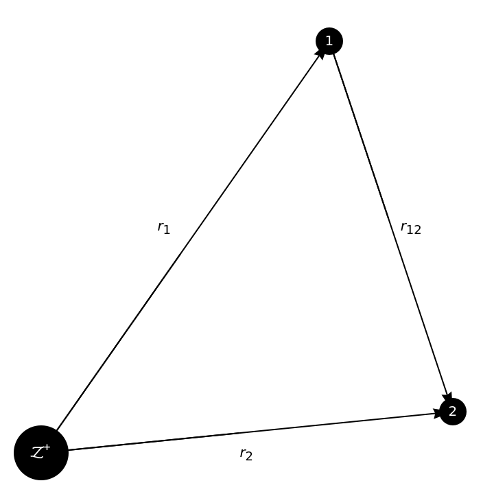
)where is the Hamiltonian, is the kinetic energy operator, and is the potential energy. The interparticle coordinates—, , and —are defined below:
ℋ
r
1
r
2
r
12
Show[Graphics[{Arrow[{{0,0},{1,0.1}}],Arrow[{{0,0},{0.7,1}}],Arrow[{{0.7,1},{1,0.1}}],AbsolutePointSize[40],Point[{0,0}],AbsolutePointSize[20],Point[{1,0.1}],Point[{0.7,1}],Text[,{0.3,0.55}],Text[,{0.5,0}],Text[,{0.9,0.55}],GrayLevel[1],Text[1,{0.7,1}],Text[2,{1,0.1}],Text[,{0,0}]}],AspectRatioAutomatic,PlotRange{{-0.1,1.1},{-0.1,1.1}}]
r
1
r
2
r
12
+
Δ
i
i
r=(r,θ,ϕ)
Δ=-(θ,ϕ),
1
2
r
∂
2
r
∂
∂r
∂r
1
2
r
2
l
(
2
)where the angular part, (θ,ϕ), is the square of the (total) angular momentum operator,
2
l
2
l
1
sin(θ)
∂sin(θ)
∂
∂θ
∂θ
1
2
sin
2
∂
∂
2
ϕ
(
3
)For spherically symmetric states (s-states), one has
Δ
1
Δ
2
1
2
r
1
∂
2
r
1
∂
∂
r
1
∂
r
1
1
2
r
2
∂
2
r
2
∂
∂
r
2
∂
r
2
1
2
r
1
1
2
r
2
2
l
(
4
)where ·=cos(θ) (i.e., is the angle between and ) and
r
1
r
2
r
1
r
2
θ
r
1
r
2
2
l
1
sin(θ)
∂sin(θ)
∂
∂θ
∂θ
(
5
)Perturbation Calculation
Perturbation Calculation
Considering the inter-electron potential, , as a perturbation, the Hamiltonian can be written as
1/
r
12
ℋ+,
-(+)--
1
2
Δ
1
Δ
2
Z
r
1
Z
r
2
(0)
ℋ
1
r
12
︸
′
ℋ
(
6
)where
(0)
ℋ
--
1
2
Δ
1
Z
r
1
ℋ
1
--
1
2
Δ
2
Z
r
2
ℋ
2
(
7
)and
′
ℋ
1
r
12
(
8
)To zeroth order, the Hamiltonian is simply separated into the sum of two single-particle (hydrogenic) operators, =+. Hence the (unnormalized) ground state of the a two-electron atom can be approximated by a product of hydrogenic functions (with nuclear charge ),
(0)
ℋ
ℋ
1
ℋ
2
Z
(0)
ψ
-Z(+)
r
1
r
2
(
9
)and the energy is the sum of the two hydrogenic (ground-state) energies, i.e.,
(0)
ℋ
(0)
ψ
(0)
ℰ
(0)
ψ
where
(0)
ℰ
2
Z
2
2
Z
2
2
Z
(
10
)1. Show that is an eigenfunction of with corresponding zeroth order energy, =-. [2]
(0)
ψ
(0)
ℋ
(0)
ℰ
2
Z
2. What is the helium ground state energy of the zeroth order approximation? Compare this to the exact value of -2.904... [2]
2.1. First-order perturbation energy
2
.1
. First-order perturbation energyThe first-order perturbation energy, , is =+Δℰ, where the energy shift is given by
(1)
ℰ
(1)
ℰ
(0)
ℰ
Δℰ=.
(0)
ψ
1
r
12
(0)
ψ
(0)
ψ
(0)
ψ
(
11
)2.2. “Standard method” for computing Δℰ
2
.2
. “Standard method” for computing Δℰ
The usual textbook computation of is as follows. We need to compute
Δℰ
(0)
ψ
1
r
12
(0)
ψ
(0)
ψ
(0)
ψ
-Z(+)
r
1
r
2
1
r
12
-Z(+)
r
1
r
2
r
1
r
2
∫∫
-2Z(+)
r
1
r
2
r
1
r
2
(
12
)Generating Function
Generating Function
Since =+-2cos(θ), we can expand the perturbation using the generating function for Legendre polynomials:
2
r
12
2
r
1
2
r
2
r
1
r
2
1
r
12
1
2
r
1
2
r
2
r
1
r
2
1
r
>
1+-2cos(θ)
2
r
<
r
>
r
<
r
>
1
r
>
∞
∑
l=0
l
r
<
r
>
P
l
(
13
)where =max(,), =min(,) and is the angle between and .
r
>
r
1
r
2
r
<
r
1
r
2
cos(θ)
r
1
r
2
Since ·cos(θ)·cos(θ) it is easy to show that
r
1
r
2
r
1
r
2
u
1
u
2
cos(θ)=cos()cos()+sin()sin()cos(-).
θ
1
θ
2
θ
1
θ
2
ϕ
2
ϕ
1
(
14
)Addition Theorem
Addition Theorem
Using the addition theorem
P
l
4π
2l+1
l
∑
m=-l
*
m
Y
l
θ
1
ϕ
1
m
Y
l
θ
2
ϕ
2
(
15
)and the orthonormality of the spherical harmonics, (θ,ϕ), the angular integrals are trivial
m
Y
l
2π
∫
0
π
∫
0
2π
∫
0
π
∫
0
P
l
θ
1
θ
1
ϕ
1
θ
2
θ
2
ϕ
2
4π
2l+1
l
∑
m=-l
2π
∫
0
π
∫
0
*
m
Y
l
θ
1
ϕ
1
θ
1
θ
1
ϕ
1
2
π
δ
l,0
δ
m,0
2π
∫
0
π
∫
0
m
Y
l
θ
2
ϕ
2
θ
2
θ
2
ϕ
2
2
π
δ
l,0
δ
m,0
2
(4π)
δ
l,0
(
16
)We have used the fact that (θ,ϕ) is a constant,
0
Y
0
In[]:=
0
Y
0
Out[]=
1
2
π
and introduced this term into both integrals so that the orthonormality condition can be applied.
3. Verify the addition theorem for . [2]
0<=l<=6
Perturbation Energy
Perturbation Energy
Hence the six-fold integration reduces to a two-dimensional integral, with the inner integral split into two cases.
=+.
(0)
ψ
1
r
12
(0)
ψ
2
(4π)
∞
∫
0
-2Z
r
1
1
r
1
r
1
∫
0
-2Z
r
2
2
r
2
r
2
∞
∫
r
1
-2Z
r
2
1
r
2
2
r
2
r
2
2
r
1
r
1
(
17
)4. Compute . [1]
ℐ=
(0)
ψ
1
r
12
(0)
ψ
5. Compute the normalization integral . [1]
=
(0)
ψ
(0)
ψ
6. Determine Δℰ. [1]
2.3. Perimetric Coordinates
2
.3
. Perimetric CoordinatesThe matrix element of a general operator, , can be computed from the integral
〈ψψ〉=∫∫ψ
*
ψ
r
12
r
1
r
2
(
18
)In interparticle coordinates this reads
〈ψψ〉=8+ψ≡8+-ψ++-ψ
2
π
∞
∫
0
∞
∫
0
r
1
r
2
∫
-
r
1
r
2
*
ψ
r
1
r
2
r
12
r
12
r
2
r
1
2
π
∞
∫
0
r
1
∫
0
r
1
r
2
∫
r
1
r
2
*
ψ
r
1
r
2
r
12
r
12
r
2
r
1
∞
∫
0
∞
∫
r
1
r
1
r
2
∫
r
2
r
1
*
ψ
r
1
r
2
r
12
r
12
r
2
r
1
(
19
)There is a simpler way: interparticle coordinates suffer from the fact that their variables satisfy triangular inequalities, , complicating the integration. This can be avoided by introducing perimetric coordinates (Coolidge and James 1937), which treat all three particles on an equal footing:
-≤<=+
r
1
r
2
r
12
r
1
r
2
with inverse:
In particular, with the exponential ansatz,
the general matrix element is trivial to compute:
Indeed, computing this matrix element integral is immediate:
Observe that
and, in general
Define this general matrix element (after moving the power of 2 to the left-hand side of the equation) as
Normalisation
Normalisation
Electron-electron interaction
Electron-electron interaction
Total energy
Total energy