CITE THIS NOTEBOOK: Wolfram R&D LIVE: Everything to Know about Mellin-Barnes Integrals - Part I by Oleg Marichev. Wolfram Community FEB 24 2023.
Introduction
Introduction
What is Mellin-Barnes integrals (MBintegrals)
What is Mellin-Barnes integrals (MBintegrals)
Pincherle S . (1888), Mellin H . (1910), Barnes E . W . (1908), Dixon A . L ., Ferrar W . L . (1936)
In Slater' type notations the MBintegral is ( sometimes)
s->
1
s
MBintegral=Gamma[+s]Gamma[-s]Gamma[+s]Gamma[-s]s(*Gamma[-s]Gamma[+s]Gamma[-s]Gamma[+s]sSimmetry*)
1
2π
γ+∞
∫
γ-∞
A
∏
k=1
a
k
α
k
B
∏
k=1
b
k
β
k
C
∏
k=1
c
k
γ
k
D
∏
k=1
d
k
δ
k
-s
z
1
2π
γ+∞
∫
γ-∞
A
∏
k=1
a
k
α
k
B
∏
k=1
b
k
β
k
C
∏
k=1
c
k
γ
k
D
∏
k=1
d
k
δ
k
s
z
α
k
β
k
γ
k
δ
k
Music, easy to remember: {A, B, C, D}, {a, b, c, d}, {α, β, γ, δ}
A+D-B-C>or<or==0(*direction'schoice*)
z
z
A+B-C-D>or==0(*sectorexisting*)
z
ℒ={γ-∞,γ+∞}(*ℒverticalorleftlooporrightloop*)
ℒ
-∞
ℒ
∞
In[]:=
,/.{z->-2,s->Random[Complex]}
s
z
-s
1
z
In[]:=
TableWith{z=Random[]Exp[PiIkk/16],s=Random[Complex]},,{kk,0,34}//Chop
s
z
-s
1
z
Out[]=
{1.,1.,1.,1.,1.,1.,1.,1.,1.,1.,1.,1.,1.,1.,1.,1.,-0.107116-0.0279068,1.,1.,1.,1.,1.,1.,1.,1.,1.,1.,1.,1.,1.,1.,1.,1.,1.,1.}
In[]:=
PowerExpand[,Assumptions->True]
b
()
a
z
2bπFloor-
1
2
Im[aLog[z]]
2π
ab
z
Out[]=
True
1
2π
γ+∞
∫
γ-∞
-s
z
2
Gamma[-s]
Gamma[1-s]
In[]:=
ResourceFunction["MeijerGForm"][Log[1+z],z]
In[]:=
System`MeijerGDump`SlaterForm[MeijerG[{{1,1},{}},{{1},{0}},z],s]
Gamma[1+s]==ComplexInfinity/;s=-1,-2,-3,…
Re[s+1]>0
In[]:=
-s
z
-s
z
2
Gamma[-s]
Gamma[1-s]
Out[]=
True
-1<γ<0
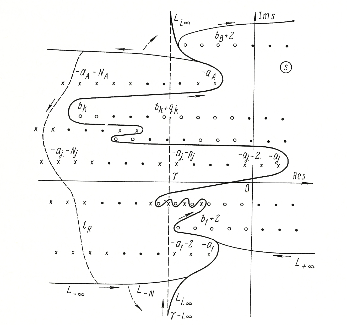
Contour ℒ for MB integrals
Contour ℒ for MB integrals
Out[]=
Example with Exp for {A,B,C,D}={1,0,0,0}
Example with Exp for {A,B,C,D}={1,0,0,0}
Poles of gamma function :
Gamma[s]==ComplexInfinity/;a->-k&&k∈Integers&&k>=0
In[]:=
Series[Gamma[s],{s,-k,1},Assumptions->{k∈Integers&&k>=0}]
Out[]=
k
(-1)
k!(s+k)
k
(-1)
k!
k
(-1)
2
π
2
PolyGamma[0,1+k]
6k!
2
O[s+k]
1
2π
γ+∞
∫
γ-∞
-s
z
-z
1
2π
γ+∞
∫
γ-∞
a
1
α
1
-s
z
-
1
α
1
z
a
1
α
1
z
α
1
In[]:=
Solve[+s==-k,s]
a
1
α
1
Out[]=
s
-k-
a
1
α
1
plus Residue :
In[]:=
ResidueGamma[+s],s,,Assumptions->{k∈Integers&&k>=0}
a
1
α
1
-s
z
-k-
a
1
α
1
Out[]=
k
(-1)
k
α
1
a
1
α
1
z
k!
α
1
In[]:=
Sum[%,{k,0,∞}]
Out[]=
-
1
α
1
z
a
1
α
1
z
α
1
Formally with 3 steps for left SIMPLE poles (for right poles we need to multiply on -1):
In[]:=
Gamma1[+s]/.s->
a
1
α
1
-s
z
-k-
a
1
α
1
Out[]=
-
-k-
a
1
α
1
z
In[]:=
%/.Gamma1[-k]->k!
k
(-1)
α
1
Out[]=
k
(-1)
-
-k-
a
1
α
1
z
k!
α
1
In[]:=
Sum[%,{k,0,∞}]
Out[]=
-
1
α
1
z
a
1
α
1
z
α
1
Example with Exp for {A,B,C,D}={0,1,0,0}
Example with Exp for {A,B,C,D}={0,1,0,0}
Important literature for beginners
Important literature for beginners
Connection with FourierTransform
Connection with FourierTransform
FourierTransform[f[t],t,z]f[t]t
1
2π
∞
∫
-∞
tz
FourierTransformf[t-τ]g[τ]τ,t,z
∞
∫
-∞
2π
FourierTransform[f[t],t,z]FourierTransform[g[t],t,z]Finally
General MBintegrals defining MeijerG & FoxH functions
General MBintegrals defining MeijerG & FoxH functions
MeijerG & generalized MeijerG https://www.wolframalpha.com/input?i=MeijerG
MeijerG & generalized MeijerG https://www.wolframalpha.com/input?i=MeijerG
Meijer C . S . (1936, 1941, 1946)
Craziness in definition of MeijerG
Craziness in definition of MeijerG
The reason is hiding in the complimentary formula for gamma function:
Evaluation of MBintegrals for MeijerG function
Evaluation of MBintegrals for MeijerG function
Main formulas for Gamma https://functions.wolfram.com/GammaBetaErf/Gamma/
Main formulas for Gamma https://functions.wolfram.com/GammaBetaErf/Gamma/
From Marichev’s book 1978
From Marichev’s book 1978
THEOREM 17 (Slater’s theorem [67, book 1966, page 57]). Let
where
then for these s we have
From pages 62 - 63 of Marichev' s book 1978 (1983)
Bearing in mind the equalities
which are deduced by using the formulae
we easily obtain the following estimate of the integrand as Re(s)∞
By applying this estimate and the first of the formulae we obtain the equality