This computational essay follows from my presentation at the Knowledge Share event organized by the Open Quantum Institute (hosted by CERN). I explored intuitive insights into the Quantum Approximate Optimization Algorithm (QAOA), focusing on the Max-Cut problem. With the symbolic tools provided by the Wolfram Quantum Framework, we can model and visualize quantum processes clearly, making complex concepts more accessible.
Understanding Quantum Approximate Optimization Algorithm (QAOA)
Understanding Quantum Approximate Optimization Algorithm (QAOA)
Load Wolfram Quantum Framework:
In[]:=
<<Wolfram`QuantumFramework`<<Wolfram`QuantumFramework`QuantumOptimization`
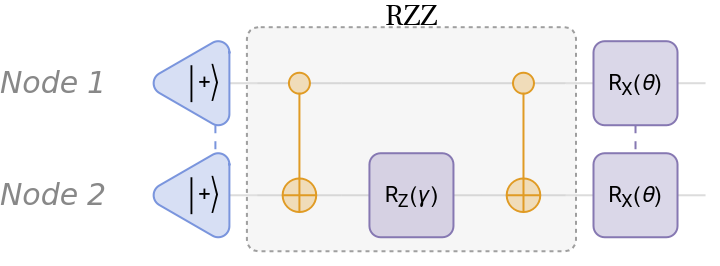
To solve the Max-Cut problem using QAOA, we define a variational ansatz consisting of RZZ entangling gates and single-qubit rotation gates:
In[]:=
rzz=QuantumCircuitOperator[{"CNOT","RZ"[γ]{2},"CNOT"},"Label"->Style["RZZ",FontSize->14]];miniQAOA=QuantumCircuitOperator[{"+"->{1,2},rzz,"RX"[θ]{1,2}}]
Out[]=
QuantumCircuitOperator

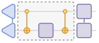
But what exactly is happening inside this circuit?
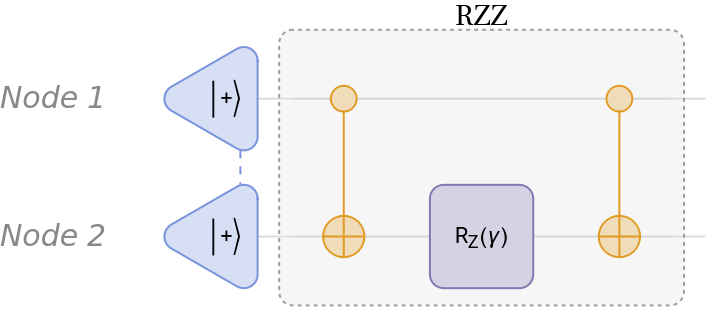
The RZZ gate encodes the connections between graph nodes, helping to identify bitstring patterns that correspond to possible solutions:
In[]:=
qc=miniQAOA[[;;2]];Row#"Diagram",,#["Simplify"]["Table"]&@qc
Out[]=
| |
|00〉 | 1 2 - γ 2 |
|01〉 | 1 2 γ 2 |
|10〉 | 1 2 γ 2 |
|11〉 | 1 2 - γ 2 |
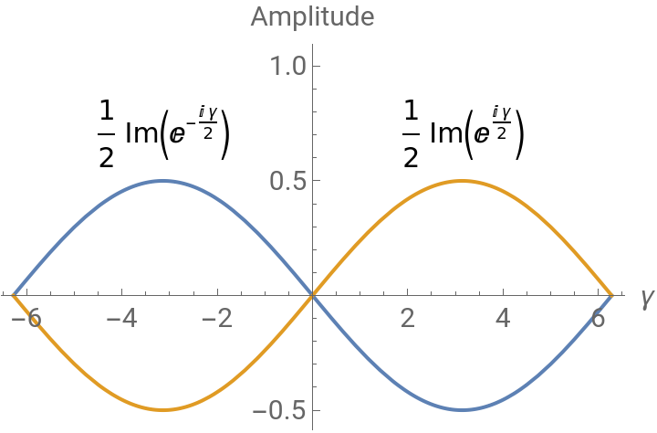
As shown in the following image, the amplitude of periodic and non-periodic bitstrings oscillate:
In[]:=
PlotEvaluate[Im[Values[#]]],{γ,-2π,2π},&@qc["Amplitudes"][[;;2]]
Out[]=


This behavior becomes even clearer when we observe the probabilities instead of amplitudes. The probability of non-periodic bitstrings vanishes as the periodic ones rise:
In[]:=
PlotEvaluate[Values[#1]/.Im[γ]γ],{γ,-2π,2π},&@qc["Probability"][[;;2]]
Out[]=
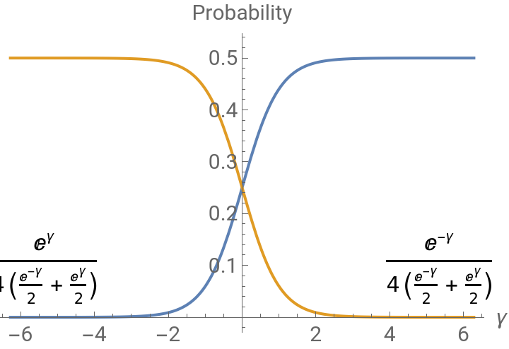
This aligns with the goal of Max-Cut: we’re looking for bitstrings that maximize edge cuts, typically, periodic patterns where nodes are in opposing sets.
However, the state produced by just the RZZ layer is too simple. To explore a richer solution space, we introduce a layer of parameterized rotations:
In[]:=
Row#"Diagram",,#["Simplify"]["Table"]&@miniQAOA
Out[]=
| |
|00〉 | - γ 2 1 2 2 Cos θ 2 1 2 2 Sin θ 2 1 2 γ 2 |
|01〉 | γ 2 1 2 2 Cos θ 2 1 2 2 Sin θ 2 1 2 - γ 2 |
|10〉 | γ 2 1 2 2 Cos θ 2 1 2 2 Sin θ 2 1 2 - γ 2 |
|11〉 | - γ 2 1 2 2 Cos θ 2 1 2 2 Sin θ 2 1 2 γ 2 |
This dramatically enhances the expressiveness of the circuit. As you’ll see in the next plot, this adds an extra dimension, creating a landscape of peaks and valleys, helping us better navigate toward optimal solutions:
In[]:=
Plot3DEvaluate[ComplexExpand@Values[#]],{γ,-2π,2π},{θ,-π,π},&@Normal[miniQAOA[]["Probabilities"][[;;2]]]
Out[]=


QAOA-in-QAOA
QAOA-in-QAOA
To tackle large graphs, we use a method called QAOA-in-QAOA, inspired by the Divide and Conquer algorithm.
Here’s the idea:
◼
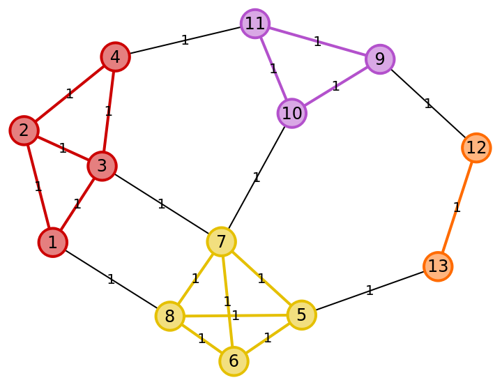
First, we partition the graph into smaller subgraphs.
◼
Next, we solve a mini-QAOA on each subgraph and combine the solutions.
◼
Then, to correct any possible issue with the solutions between the subgraphs, we treat each subgraph as a node in a new coarse-grained graph.
◼
Finally, we apply QAOA again to this higher-level graph and correct the final solution.
This process is recursive and scalable, making it suitable for large problem instances.
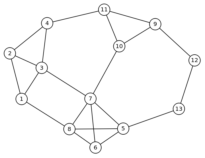
Now let’s see how the Wolfram Quantum Framework enables us to symbolically model and analyze this algorithm. Given the following graph:
In[]:=
1=UndirectedEdge@@@{{1,2},{2,3},{3,4},{2,4},{1,3}};2=UndirectedEdge@@@(4+{{1,2},{2,3},{3,4},{1,4},{2,4},{1,3}});3=UndirectedEdge@@@(8+{{1,2},{2,3},{3,1}});4=UndirectedEdge@@@(11+{{1,2}});connection=UndirectedEdge@@@{{4,11},{10,7},{9,12},{13,5},{3,7},{1,8}};edges={1,2,3,4};fullEdges=Flatten[{{4,2,1,3},connection}];g=Graph[fullEdges,PlotTheme"NameLabeled",EdgeWeightThread[fullEdges1]]
Out[]=
Given the following partition:
In[]:=
subgraphs=Graph#,EdgeWeight->Thread[Rule[#,1]],&/@edges;gsub=HighlightGraphfullEdges,subgraphs,
Out[]=
Divide (Subgraphs)
Divide (Subgraphs)
We load the Hamiltonian for each minigraph:
We then construct symbolic QAOA circuits, with qubit indices mapping directly to graph nodes:
After simulating the states, we can observe how the symbolic computation can give insights about cost functions for each subgraph. We can visualize the parameter space using contour plots, giving us deep insight into the optimization behavior.
After just a single QAOA layer, we already discover useful solutions:
Each minigraph contributes to a partial solution, illustrated by colored nodes yellow and red:
Conquer (Big graph)
Conquer (Big graph)
In the Conquer phase, we construct a new graph where each node represents a subgraph, and the edges are based on their prior connections:
We then assign weights based on inter-subgraph interactions and repeat the QAOA process at this higher level:
Finally, we observe the resulting probability distribution and solve the MaxCut problem for the higher-level graph:
n the final step, we take the subgraphs that are yellow nodes in the higher level graph and flip their node values. For instance, in some subgraphs, yellow nodes may become red, as the global optimization balances local and global constraints.
References
References
◼
Zhou, Z., Du, Y., Tian, X., & Tao, D. (2023). QAOA-in-QAOA: Solving Large-Scale MaxCut Problems on Small Quantum Machines. Physical Review Applied, 19(2).
https://doi.org/10.1103/physrevapplied.19.024027
https://doi.org/10.1103/physrevapplied.19.024027
◼
Esposito, A., & Danzig, T. (2024). Hybrid Classical-Quantum Simulation of MaxCut using QAOA-in-QAOA. In 2024 IEEE International Parallel and Distributed Processing Symposium Workshops (IPDPSW) (pp. 1088–1094).
https://doi.org/10.1109/ipdpsw63119.2024.00180
https://doi.org/10.1109/ipdpsw63119.2024.00180
CITE THIS NOTEBOOK
CITE THIS NOTEBOOK
Symbolic methods in quantum optimization: introduction to QAOA-in-QAOA
by Sebastian Rodriguez
Wolfram Community, STAFF PICKS, May 16, 2025
https://community.wolfram.com/groups/-/m/t/3462606
by Sebastian Rodriguez
Wolfram Community, STAFF PICKS, May 16, 2025
https://community.wolfram.com/groups/-/m/t/3462606