A string rewriting rule becomes a linear operator when words are promoted to basis vectors. Commutators of such operators generate familiar Lie algebras: sl₂, the one-sided Witt algebra, and the Heisenberg algebra. This structure lifts to Hyperstrings, directed graphs that encode sets of words. Computational experiments in Mathematica reveal the correspondence and an open puzzle about confluence diamonds.
Imagine starting with the word abba and a simple rule: whenever you see ab, swap it to ba. If we swap the first two letters of abba, we get baba. There is still an ab in the middle, so we swap it again to get bbaa. Since there are no more ab’s left, the game has to stop. This is a basic letter-swapping game, but even with just one rule, things quickly get interesting.
This simple game raises some fundamental questions. Does the game always stop [1]? How many moves does it take? Does the order of our moves matter, and do we get the same answers if we change the rule slightly? To approach these questions in a controlled way, we need to see what kinds of mathematical structures show up as we play.
This simple game raises some fundamental questions. Does the game always stop [1]? How many moves does it take? Does the order of our moves matter, and do we get the same answers if we change the rule slightly? To approach these questions in a controlled way, we need to see what kinds of mathematical structures show up as we play.
Part I: From String Rewriting Rules to Lie Algebras
String Rewriting Rules as Linear Operators
String Rewriting Rules as Linear Operators
Let’s turn our rewriting rule into linear algebra. We can do this by promoting each word to a state [2]. Specifically, a basis vector in a vector space. This lifts our rule to a linear operator . Now, rewriting behaves like a non-deterministic dynamical system, where the operator acts as a vector field over the space of words, generating an infinitesimal transformation.This translation makes the concept of fixed points remarkably clean. Classically, a fixed point is a “no-match” string where . Linearly, this condition simply becomes |S〉=0, the operator annihilates any string with no match. To make this concrete, we construct our system on , the vector space spanned by all words over an alphabet of length at most .
R
S
|S〉
R
R
R
S
R(S)=S
R
≤n
V
n
For simplicity, we will drop the ket notation, but keep in mind we are dealing with states, not strings. The rule acts as a linear operator on the free vector space spanned by length- words over the alphabet , mapping each word to the formal sum of all words you get by rewriting one occurrence of to .
Because this operator eats words of length and the rule changes the length by , it spits out words of length . We can think of our letters as basis vectors of . Since a word is just the tensor product of its letters, the length- words form a basis for . Under this view, a rewrite rule becomes a matrix.
wv
n
A
w
v
Because this operator eats words of length
n
|v|-|w|
n+|v|-|w|
d
n
⊗n
()
d
To see this in action, look at the rules on the left. Here, is the length of the input words. The rule matrix represents our rewriting rule as a linear operator on the free vector space of words over our alphabet . Choosing simply fixes the graded piece of the space we are acting on. On the right, you can see the resulting matrix representation, with the basis elements explicitly labeled.
n
wv
a
n
Out[]=
AB, a = {A,B}, n = 2 |
| ||||||||||||||||||||||||||||||||||||||||||||||||||||||||||||||||||||||||||||||||||||||||||||||||||||
AB, a = {A,B,C}, n = 2 |
| ||||||||||||||||||||||||||||||||||||||||||||||||||||||||||||||||||||||||||||||||||||||||||||||||||||
AAA, a = {A,B}, n = 2 |
| ||||||||||||||||||||||||||||||||||||||||||||||||||||||||||||||||||||||||||||||||||||||||||||||||||||
AAA, a = {A,B}, n = 3 |
|
On single letters, the operator sends to and annihilates , meaning a word with no match maps to zero, not to itself.
Now, the tensor product⊗ rewrites both positions of a two-letter word at the same time, sending to .
This is different from our full rule matrix, which sums over match positions. For example, applying to yields the superposition . This sum over positions is what makes rule matrices act as derivations rather than simple substitutions, and it is the source of the non-trivial commutators we will see below.
R
AB
A
B
B
Now, the tensor product
R
AB
R
BA
A⊗B
B⊗A
This is different from our full rule matrix, which sums over match positions. For example, applying
AB
AA
AB+BA
Out[]=
A | = |
| |||||||||||||||||||||||||||
B | = |
| |||||||||||||||||||||||||||
AB = A⊗B | = |
| = e₂ | ||||||||||||||||||||||||||
R AB | = |
| |||||||||||||||||||||||||||
R AB | = |
| = |
| no match → 0 | ||||||||||||||||||||||||
R AB R BA | = |
| |||||||||||||||||||||||||||
( R AB R BA | = |
| = |
| = BA = e₃ | ||||||||||||||||||||||||
R AB | = |
| = |
| = AB + BA : sum over match positions | ||||||||||||||||||||||||

A rule with length change is a graded operator: it maps length- words to length words. When we take the commutator of a degree- and a degree- operator, each factor evaluates at the correct intermediate length. This ensures both products map to , so they share the same, possibly rectangular, shape. The bracket is square only when .Four examples follow. First, length-preserving rules on single letters recover , and this same bracket at acts diagonally with eigenvalue . Second, bracketing a length-raising rule with a length-preserving one gives a rectangular, degree-1 commutator. Finally, a raising and lowering pair returns us to degree 0, with diagonal entries that count overlapping matches.
p=|v|-|w|
n
n+p
p
q
⊗n
()
d
⊗(n+p+q)
()
d
p+q=0
[,]=-
E
12
E
21
E
22
E
11
n=2
#B-#A
Out[]=
| ||||||||||||||||||||||||||||||||||||||||||||||||||||||||||||||||||||||||||||||||||||||||||||||||||||
| ||||||||||||||||||||||||||||||||||||||||||||||||||||||||||||||||||||||||||||||||||||||||||||||||||||
| ||||||||||||||||||||||||||||||||||||||||||||||||||||||||||||||||||||||||||||||||||||||||||||||||||||
| ||||||||||||||||||||||||||||||||||||||||||||||||||||||||||||||||||||||||||||||||||||||||||||||||||||
The Lie Algebra Search
The Lie Algebra Search
Our search separates into two distinct regimes. Brackets of rules like and keep producing longer and longer words, so the operators never stop generating new ones: the algebra is infinite-dimensional. Finite-dimensional algebras appear only when the growth is cut off, words beyond a fixed length are quotiented to zero.
One infinite family can be handled exactly: the rules generate the one-sided Witt algebra, proven by hand (proof not shown here); the section below exhibits the structure computationally.
a
m
a
a
n
a
One infinite family can be handled exactly: the rules
a
k+1
a
Roots and the Weight Lattice
Roots and the Weight Lattice
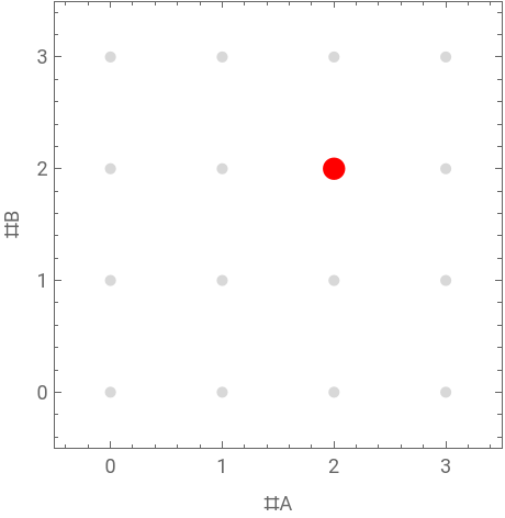
We can project words in the alphabet to the lattice by counting their letters [3]: each word maps to its weight . The first picture shows the weight of the word at the point , while the board lists the full weight space at all six words with two ’s and two ’s.
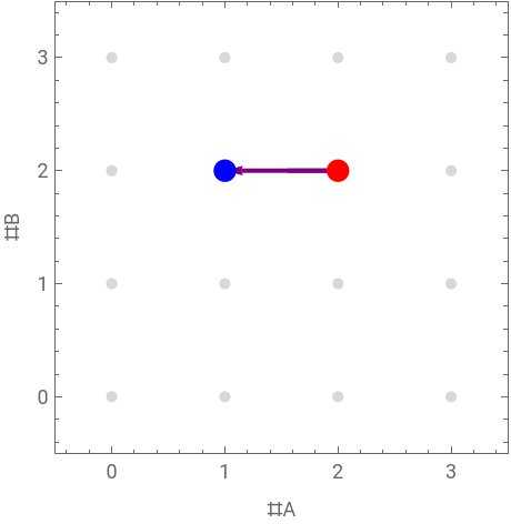
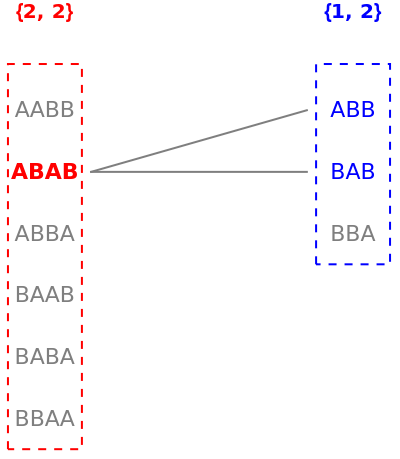
A rewrite rule shifts every word’s letter count by the same fixed vector, . This vector acts as a root: on the lattice, the rule simply translates weights, shown by the arrow from to . The last panel shows the rule acting directly on words. Because contains the pattern at two positions, the rule maps it to two words, and , both of weight . Here in the lattice, the rule is a simple translation.
{A,B}
2
(#A,#B)
ABAB
(2,2)
(2,2),
A
B
A rewrite rule
ABB
(-1,0)
(2,2)
(1,2)
ABAB
AB
BAB
ABB
(1,2)
Out[]=

Weight space at {2, 2} |
With this setup, we can ask some fascinating questions. Can we find rules that satisfy ? Our target is a set of at least three rules where every pairwise bracket yields a scalar multiple of a single rule in the set, with no general linear combinations allowed. This condition is much stricter than the usual closure studied in rule algebras. For instance, a set like closes as a linear span, but it fails our test because - is not a single rule.To find these sets, we filter before we search. Each rule can be a vector, which is the net change in letter counts . Because the bracket is additive on weights, the relation forces the weights to add up, meaning . This simple arithmetic condition filters away most candidate triples before we compute a single commutator, leaving only a few surviving clusters to test exhaustively.We run our search over all rules over alphabets of size 1, 2, and 3, restricting the input length and the output length . We partition the search space by alphabet size.
,=γ
R
i
R
j
R
k
{,,-}
E
ab
E
ba
E
bb
E
aa
E
bb
E
aa
(Δ#A,Δ#B,Δ#C)∈
|alphabet|
,=γ
R
i
R
j
R
k
wt()=wt()+wt
R
k
R
i
R
j
uv
|u|∈{1,2,3}
|v|∈{0,1,2,3}
Alphabet {A}
Alphabet {A}
The two search cells below were generated with AI assistance (Claude Fable 5) . The reported witnesses were confirmed by independent runs, but the author has not audited the search code line by line . Readers are welcome to run, modify, and stress - test it .
Alphabet {A, B}
Alphabet {A, B}
We establish an explicit certificate: any candidate rule must have a footprint of at most 6, which bounds the search.
Alphabet {A, B, C}
Alphabet {A, B, C}
Everything so far acts on one string at a time. A rule takes a word, finds a match, and produces another word, with the operators of Part I organized sector by sector and length by length. But the objects of real interest are often sets of words, such as the reachable states of a rewriting system, the value sets of a computation, or a formal language. This raises a natural question: is there a single finite object that carries a whole family of strings at once, on which rewriting can act directly?
There is: a hyperstring, which is a directed acyclic graph whose paths spell words. The rest of this essay develops hyperstrings, shows that rewriting them matches rewriting every individual string they carry, and verifies that the Lie algebra structure of Part I survives this lift intact.
There is: a hyperstring, which is a directed acyclic graph whose paths spell words. The rest of this essay develops hyperstrings, shows that rewriting them matches rewriting every individual string they carry, and verifies that the Lie algebra structure of Part I survives this lift intact.
Part II: Hyperstring
Definition of a Hyperstring
Definition of a Hyperstring
Mapping Between Strings and Hyperstrings
Mapping Between Strings and Hyperstrings
Claim:
HyperstringToStrings ∘ StringsToHyperstring is the identity on nonempty finite string sets.
Hence StringsToHyperstring is injective, HyperstringToStrings is surjective, and each string set L is recovered exactly from the hyperstring built from it:
HyperstringToStrings ∘ StringsToHyperstring is the identity on nonempty finite string sets.
Hence StringsToHyperstring is injective, HyperstringToStrings is surjective, and each string set L is recovered exactly from the hyperstring built from it:
Witnesses of the claim:
Witnesses of the claim:
For all nonempty finite L, HyperstringToStrings(StringsToHyperstring(L)) = L:
StringsToHyperstring(L₁) = StringsToHyperstring(L₃) ⟹ L₁ = L₃:
For every L there exists H with HyperstringToStrings(H) = L:
Hyperstring Rewriting Rules
Hyperstring Rewriting Rules
Rules as graph pairs
Rules as graph pairs
Matching and applying a rule
Matching and applying a rule
Two Ways to Rewrite: Fresh or Shared Vertices
Two Ways to Rewrite: Fresh or Shared Vertices
Sliced Rewriting
Sliced Rewriting
Pushforward: The Lie Algebra Structure Lifts to Hyperstrings
Pushforward: The Lie Algebra Structure Lifts to Hyperstrings
The Commuting Square
The Commuting Square
Route 1: Hyperstring, Rewrite, Then Read Off Words
Route 1: Hyperstring, Rewrite, Then Read Off Words
H:
moving along the upper arrow to R(H):
moving down to HyperstringToString(R(H)):
Route 2: Hyperstring, Read Off Words, Then Rewrite
Route 2: Hyperstring, Read Off Words, Then Rewrite
moving down from H to HyperstringToString(H):
Lie Structure on Hyperstrings
Lie Structure on Hyperstrings
Recall
Recall
One-Sided Witt
One-Sided Witt
Heisenberg
Heisenberg
Final thoughts: Diamonds, An Open Puzzle
Final thoughts: Diamonds, An Open Puzzle
Now let' s look at a random Hyperstring over the alphabet {X, Y, Z}:
• Why does the shared mode have fewer diamonds overall?
• How do asymmetric diamonds form only in fresh mode?
• How can we have an arm of length 4 at depth 3?
• ...
• How do asymmetric diamonds form only in fresh mode?
• How can we have an arm of length 4 at depth 3?
• ...
While commutators show us which rules generate which Lie algebras, and the pushforward proves this structure survives the transition from strings to Hyperstrings, the diamonds are counting something else: not what the operators are, but how their applications interleave and collide [1] [7].
Whether that geometry can be organized by an algebraic invariant of its own, or whether it reflects a purely combinatorial behavior that no bracket can capture, remains open. All of the code in this notebook is self-contained; any reader with a spare afternoon and a fresh kernel is warmly invited to find out.
Whether that geometry can be organized by an algebraic invariant of its own, or whether it reflects a purely combinatorial behavior that no bracket can capture, remains open. All of the code in this notebook is self-contained; any reader with a spare afternoon and a fresh kernel is warmly invited to find out.
Acknowledgements
Acknowledgements
The author thanks Stephen Wolfram for proposing the term Hyperstring, and Pavel Hajek for his guidance, mathematical inspiration, and helpful discussions.
References
References
[1] M. H. A. Newman (1942), “On Theories with a Combinatorial Definition of ‘Equivalence’,” Annals of Mathematics 43(2), 223–243.
[2] N . Behr, V . Danos and I . Garnier (2016), "Stochastic Mechanics of Graph Rewriting," Proceedings of the 31 st Annual ACM/IEEE Symposium on Logic in Computer Science (LICS' 16), 46–55. https : // doi . org/10.1145/2933575.2934537
[3] W. Fulton and J. Harris (1991), Representation Theory: A First Course, Graduate Texts in Mathematics 129. Springer-Verlag.
[4] P. Hajek (2025), “Lie Brackets on Hypergraphs,” Wolfram Community. https://community.wolfram.com/groups/-/m/t/3358052
[5] S. Wolfram (2020), “A Class of Models with the Potential to Represent Fundamental Physics,” Complex Systems 29(2), 107–536. https://doi.org/10.25088/ComplexSystems.29.2.107
[6] P. Blasiak, G. H. E. Duchamp, A. I. Solomon, A. Horzela and K. A. Penson (2010), “Combinatorial Algebra for Second-Quantized Quantum Theory,” Advances in Theoretical and Mathematical Physics 14(4), 1209–1243. https://arxiv.org/abs/1001.4964
[7] G. M. Bergman (1978), “The Diamond Lemma for Ring Theory,” Advances in Mathematics 29(2), 178–218.
AI Disclosure
AI Disclosure
The following generative AI tools were used in this project: Claude Fable 5 (Anthropic). It was used for brainstorming, reference search, debugging code, and editing prose. All written content and code was reviewed, tested, and approved by the author, with one exception: the two exhaustive search cells in Part I (alphabet sizes 2 and 3) were reviewed and their outputs spot checked, but are provided primarily as exploratory code for readers to run and modify rather than as verified results.
CITE THIS NOTEBOOK
CITE THIS NOTEBOOK
Lie Algebras from Strings to Hyperstrings
by Sally Li
Wolfram Community, STAFF PICKS, July 16, 2026
https://community.wolfram.com/groups/-/m/t/3762249
by Sally Li
Wolfram Community, STAFF PICKS, July 16, 2026
https://community.wolfram.com/groups/-/m/t/3762249