ABSTRACT (original article): We present a generalized mathematical model for predicting the transport properties of a quantum system exposed to a stationary magnetic field and a high-intensity electromagnetic field. The new formulation, which applies to two-dimensional (2D) dressed quantum Hall systems, is based on Landau quantization theory and the Floquet-Drude conductivity approach. We model our system as a two-dimensional electron gas (2DEG) that interacts with two external fields. To analyze the strong light coupling with the 2DEG, we employ the Floquet theory as a nonperturbative procedure. Moreover, the Floquet-Fermi golden rule is adopted to explore the impurity scattering effects on charge transport in disordered quantum Hall systems. We derive fully analytical expressions to describe longitudinal components in the conductivity tensor in dressed quantum Hall systems. Subsequently, we demonstrate that the conductivity characteristics of quantum Hall systems can be manipulated using strong external light. Our results align with well-established and experimentally verified theoretical descriptions for undressed systems while providing a more generalized analysis of the conductivity characteristics in quantum Hall systems. Thus our model can be applied to accurately interpret the usage of strong external radiation as a tool in nanoscale quantum devices. CITATION (original article): Herath, K., & Premaratne, M. (2022). Generalized model for the charge transport properties of dressed quantum Hall systems. Physical Review B, 105, 035430. https://doi.org/10.1103/PhysRevB.105.035430
Introduction
Introduction
In this paper, we introduce a generalized mathematical model for predicting the transport properties of a quantum system exposed to a stationary magnetic field and a high-intensity electromagnetic field. This new model, which applies to two-dimensional (2D) dressed quantum Hall systems, is based on Landau quantization theory and the Floquet-Drude conductivity approach. In this study, we explicitly calculate the longitudinal components , ) of the conductivity tensor in a periodically driven quantum Hall system by developing a generalized analytical description using the Floquet-Drude conductivity. The derived analytical expression is further analyzed numerically using empirical system parameters to compare with the results from previous charge transport studies on quantum Hall systems.
(
σ
xx
σ
yy
Numerical Calculations
Import packages and define global parameters
Import packages and define global parameters
Import external libraries and define global parameters for images.
In[]:=
ClearAll["Global`*"]<<MaTeX`Needs["CustomTicks`"];imageScale=72/2.54;
System parameter analysis
System parameter analysis
Constants
Constants
Define common constants.
e=Quantity[(1.602176)*10^(-19),"Coulombs"];(*electron'scharge*)hbar=Quantity[(1.054571)*10^(-34),("Kilograms"*"Meters"^2)/"Seconds"];(*Plank'sconstant*)m=Quantity[(9.109383)*10^(-31),"Kilograms"];(*electron'smass*)c=Quantity[(2.997924)*10^(8),"Meters"/"Seconds"];(*speedoflightinvacuum*)ϵ0=Quantity[(8.854187)*10^(-12),("Coulombs"^2*"Seconds"^2)/("Kilograms"*"Meters"^(3))];(*vacuumpermittivity*)eV=Quantity[(1.602176)*10^(-19),("Kilograms"*"Meters"^2)/("Seconds"^(2))];(*electronVolts*)
System parameters
System parameters
Define system parameters.
In[]:=
B=Quantity[(1.2),"Kilograms"/("Coulombs"*"Seconds")];(*Stationarymagneticfield'samplitude=1.2T*)ElecInt0=Quantity[(1)*10^(6),"Kilograms"/"Seconds"^(3)];(*Referencedressingelectricfield'sintensity=100*)ω=Quantity[(2)*10^(12),"Seconds"^(-1)];(*Dressingfield'sfrequency=2×*)me=0.071*m;(*Effectiveelectron'smassfor2DEG=0.071m*)
-2
Wcm
12
10
-1
rads
Parameter calculation
Parameter calculation
Calculate required parameters.
In[]:=
ω0=(e*B)/(me);(*cyclotronfrequency*)E0=Sqrt[(2*ElecInt0)/(c*ϵ0)];(*Referencedressingelectricfield'samplitude*)b=(e*E0*((ω0)^2))/(hbar*ω*((ω0)^2-(ω)^2));(*Pre-definedparameter*)κ=Sqrt[me*ω0/hbar];(*Pre-definedparameterinGauss-Hermitefunctions*)λs1=(hbar*b)/(e*B)(*Pre-definedparameterininversescatteringtime*)λs2=(hbar*κ)/(e*B)(*Pre-definedparameterininversescatteringtime*)
Out[]=
Out[]=
Parameter values
Parameter values
Display special parameters.
In[]:=
k0=Quantity[1*10^(8),"Meters"^(-1)];
In[]:=
λ1=N[λs1*k0]
Out[]=
2.08959
In[]:=
λ2=N[λs2*k0,4]
Out[]=
2.34203
Landau level wavefunction χN
Landau level wavefunction
χ
N
Define wavefuntion of electron in a dressed Landau level.
In[]:=
χ[y_?NumericQ,N_?NumericQ]:=*N!*HermiteH[N,y];
Exp
-
2
y
2
N
2
π
We can define normalized dressed electric field intensity = ElecInt := where ElecInt0 = .
Realelectricfieldintensity
ElecInt0
100
-2
Wcm
Inverse scattering time matrix central element analysis (l=0)
Inverse scattering time matrix central element analysis (l=0)
For each Landau level, we need to calculate the central element of the inverse scattering time matrix. Here, we calculate the normalized inverse scattering time matrix’s central element.
Landau level N=0
Landau level N=0
In[]:=
Q0:=χ[λ2*k2,0]*χ[λ2*(k1-k2),0];A0[k1_?NumericQ,ElecInt_?NumericQ]:=((BesselJ[0,λ1*Sqrt[ElecInt]*(k1)])^2)*((NIntegrate[Q0,{k2,-Infinity,Infinity},AccuracyGoal4])^2);Sup0:=NIntegrate[A0[k1,eInt],{k1,-Infinity,Infinity},AccuracyGoal4];Sdown0:=NIntegrate[A0[k1,0],{k1,-Infinity,Infinity},AccuracyGoal4];Tinverse0:=Sup0/Sdown0;
Landau level N=1
Landau level N=1
In[]:=
Q1:=χ[λ2*k2,1]*χ[λ2*(k1-k2),1];A1[k1_?NumericQ,ElecInt_?NumericQ]:=((BesselJ[0,λ1*Sqrt[ElecInt]*(k1)])^2)*((NIntegrate[Q1,{k2,-Infinity,Infinity},AccuracyGoal4])^2);Sup1:=NIntegrate[A1[k1,eInt],{k1,-Infinity,Infinity},AccuracyGoal4];Sdown1:=NIntegrate[A0[k1,0],{k1,-Infinity,Infinity},AccuracyGoal4];Tinverse1:=Sup1/Sdown1;
Landau level N=2
Landau level N=2
In[]:=
Q2:=χ[λ2*k2,2]*χ[λ2*(k1-k2),2];A2[k1_?NumericQ,ElecInt_?NumericQ]:=((BesselJ[0,λ1*Sqrt[ElecInt]*(k1)])^2)*((NIntegrate[Q2,{k2,-Infinity,Infinity},AccuracyGoal4])^2);Sup2:=NIntegrate[A2[k1,eInt],{k1,-Infinity,Infinity},AccuracyGoal4];Sdown2:=NIntegrate[A0[k1,0],{k1,-Infinity,Infinity},AccuracyGoal4];Tinverse2:=Sup2/Sdown2;
Landau level N=3
Landau level N=3
In[]:=
Q3:=χ[λ2*k2,3]*χ[λ2*(k1-k2),3];A3[k1_?NumericQ,ElecInt_?NumericQ]:=((BesselJ[0,λ1*Sqrt[ElecInt]*(k1)])^2)*((NIntegrate[Q3,{k2,-Infinity,Infinity},AccuracyGoal4])^2);Sup3:=NIntegrate[A3[k1,eInt],{k1,-Infinity,Infinity},AccuracyGoal4];Sdown3:=NIntegrate[A0[k1,0],{k1,-Infinity,Infinity},AccuracyGoal4];Tinverse3:=Sup3/Sdown3;
Landau level N=4
Landau level N=4
In[]:=
Q4:=χ[λ2*k2,4]*χ[λ2*(k1-k2),4];A4[k1_?NumericQ,ElecInt_?NumericQ]:=((BesselJ[0,λ1*Sqrt[ElecInt]*(k1)])^2)*((NIntegrate[Q4,{k2,-Infinity,Infinity},AccuracyGoal4])^2);Sup4:=NIntegrate[A4[k1,eInt],{k1,-Infinity,Infinity},AccuracyGoal4];Sdown4:=NIntegrate[A0[k1,0],{k1,-Infinity,Infinity},AccuracyGoal4];Tinverse4:=Sup4/Sdown4;
Generating figures
Generating figures
Using calculated normalized inverse scattering time matrix we can generate figure fr each Landau level as follows.
In[]:=
P1=Plot[{Sqrt[Tinverse0],Sqrt[Tinverse1],Sqrt[Tinverse2],Sqrt[Tinverse3],Sqrt[Tinverse4]},{eInt,0,9},PlotRange{{0,9},{0.4,1.1}},PlotLegends{MaTeX["N=1",FontSize17],MaTeX["N=2",FontSize17],MaTeX["N=3",FontSize17],MaTeX["N=4",FontSize17],MaTeX["N=5",FontSize17]},MaxRecursion0,PlotPoints40,AxesFalse,Frame{{True,True},{True,True}},FrameTicksStyle{{FontSize18,None},{FontSize18,None}},FrameTicks{{LinTicks[{0.5,0.7,0.9,1.1},Range[0.4,1.1,0.02]],None},{LinTicks[{0,2,4,6,8},Range[0,9,0.5]],None}},FrameLabel{{MaTeX["\\Lambda_{N}",FontSize17],None},{MaTeX["I(100~\\text{W}\\text{cm}^{-2})",FontSize17],None}},ImageSize12*imageScale]
Out[]=
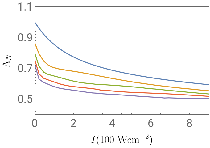


To identify the relationship between normalized inverse scattering time matrix central element with x-directional momentum component, we generate following figure (for a given dressing field’s intensity level:
Manipulate conductivity using dressing field intensity
Manipulate conductivity using dressing field intensity
Normalized conductivity function:
Getting sum of each Landau level contribution to the conductivity:
Generating figures:
Generating figures:
Calculate normalized longitudinal conductivity component for 3rd Landau level with different dressing filed intensity levels:
Calculate normalized longitudinal conductivity component for few Landau levels with different dressing filed intensity levels:
Export figures
Export figures
Export the generated figures as PDF files.
CITE THIS NOTEBOOK
CITE THIS NOTEBOOK
Generalized model for transport properties of dressed quantum Hall systems
by Kosala Herath
Wolfram Community, STAFF PICKS, March 4, 2022
https://community.wolfram.com/groups/-/m/t/2484684
by Kosala Herath
Wolfram Community, STAFF PICKS, March 4, 2022
https://community.wolfram.com/groups/-/m/t/2484684