Introduction
Introduction
In the same vein as my previous post on the fluxional molecule bullvalene, I wanted to depict the Berry pseudorotation of a trigonal bipyramidal molecule in Mathematica. Recall that the trigonal bipyramidal geometry is the molecular geometry adopted by molecules of the form according to valence shell electron pair repulsion (VSEPR) theory. A typical example is phosphorus pentachloride ), which we will be looking at for the rest of this post:
AX
5
(
PCl
5
Molecule["phosphorus pentachloride"]//MoleculePlot3D

One distinguishes between “axial” (sometimes also called “apical”) and “equatorial” ligands in a trigonal bipyramidal molecule. The three ligands that share a plane with the central atom, and are at 120° angles to each other are the equatorial ligands, while the two ligands positioned above and below that plane are the axial ligands:
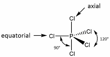
When all five ligands are identical, the axial bond lengths tend to be longer, because the axial ligand is not able to approach the central atom as closely as the ligands in equatorial position. For the specific case of phosphorus pentachloride, the axial P-Cl bond length is 2.14 Å, while the equatorial bond length is 2.02 Å.
R.S. Berry, in a 1960 paper, was able to show that the supposedly non-equivalent positions in a trigonal bipyramidal molecule undergo a positional exchange where one equatorial ligand is held fixed, and the remaining two equatorial ligands swap with the two axial ligands. This was based on spectroscopic observations (NMR, Raman, etc.) that show that all five ligands are indistinguishable. He termed this exchange between axial and equatorial ligands a “pseudorotation”, through the following mechanism depicted in his paper:
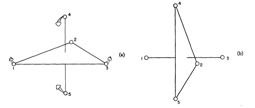
That is, trigonal bipyramidal molecules are fluxional molecules: molecules that undergo a motion such that the dynamic atoms are effectively symmetry-equivalent.
Cass, Hii, and Rzepa had previously used Jmol to depict Berry pseudorotation as featured on their Web page. I had wanted to try doing a similar visualization in Mathematica based on MoleculePlot3D, which led to the current post. (See also this survey paper by Ugi et al. for discussion on other aspects of the Berry pseudorotation.)
Simulating a pseudorotation
Simulating a pseudorotation
To facilitate the depiction of the Berry pseudorotation, I had prepared a Molecule of phosphorus pentachloride with idealized coordinates:
pcl5=Uncompress["1:eJxTTMoPSmNmYGAo5gASvvk5qcmlOalpbCARFiDhk1lcksYI4zmW5OcGg3gBaGJMQIZzDk0EWVGcwgTjOeXnpSB4ILlMkDcyQWYEg5wfnJmXDvQJPg0gtZlMpGpgIVUDK6ka2NA0MDJgDYIgYEwV80ODyzk/vyglMy+xJLUYop4XSASWJuaVZJZUOhYVJVZCNMqBjC0pKk0uKS1KTQFLJCD4Lokliagu8gQZZgYmjSEJBSaTClIHciVIlBDQjOk/9FWDwQHG/8d/5VjO39/2EPEP+9HE96OLowP51teBO+QYHXCIHwjmBIVLXnpxSVF+bjGql1DDExzkaEIg5QB785iU"]
Molecule


Verify that the axial and equatorial bond lengths are as expected:
MoleculeValue[pcl5,"BondLength"]
,,,,
Verify that the axial and equatorial bond angles are as expected:
MoleculeValue[pcl5,{"BondAngle",{{2,1,3},{3,1,4},{4,1,2},{5,1,2},{6,1,2}}}]
,,,,
As a warm-up, let us depict a single Berry pseudorotation. The implementation is fairly elaborate, since the four dynamic ligands undergo separate motions (rotations by 30° along with rescaling), implemented using the various geometric transforms available in Mathematica. (One would normally use MoleculeModify[“TransformAtomCoordinates”] if all atoms are undergoing the same transformation.) The overall operation effectively orients the molecule on its side, with the new axial ligands parallel to the plane containing the original equatorial ligands.
With[{n=16},mt=MoleculeModify[pcl5,{"RenumberAtoms",{1,4,5,6,2,3}}];coords=QuantityMagnitude[MoleculeValue[mt,"AtomCoordinates"],"Angstroms"];x1=Normalize[coords[[2]]];x2=Normalize[coords[[3]]];x3=Cross[x1,x2];f0=Table[Molecule[mt,AtomCoordinates->QuantityArray[Join[Take[coords,2],ScalingTransform[{1,1,1}Rescale[r/n,{0,1},{1,2.02/2.14}]][{RotationTransform[π/6r/n,x3][coords[[3]]],RotationTransform[-π/6r/n,x3][coords[[4]]]}],ScalingTransform[{1,1,1}Rescale[r/n,{0,1},{1,2.14/2.02}]][{RotationTransform[π/6r/n,x2][coords[[5]]],RotationTransform[-π/6r/n,x2][coords[[6]]]}]],"Angstroms"]],{r,n}]];ListAnimate[MoleculePlot3D[#,PlotRange->2.7,ViewPoint->{1.3,-2.4,0.5}]&/@Prepend[f0,mt],AnimationRunning->False]

For the final visualization, we successively depict three Berry pseudorotations, corresponding to the three possible equatorial ligands that can be held fixed. We also apply an overall 90° rotation to the molecule, to restore the “pseudorotated” result to the same orientation as the original. All of these considerations result in the following code:
With[{n=16},mt=MoleculeModify[pcl5,{"RenumberAtoms",{1,2,5,6,3,4}}];coords=QuantityMagnitude[MoleculeValue[mt,"AtomCoordinates"],"Angstroms"];x1=Normalize[coords[[2]]];x2=Normalize[coords[[3]]];x3=Cross[x1,x2];f1=Table[Molecule[mt,AtomCoordinates->QuantityArray[RotationTransform[π/2r/n,x1][Join[Take[coords,2],ScalingTransform[{1,1,1}Rescale[r/n,{0,1},{1,2.02/2.14}]][{RotationTransform[π/6r/n,x3][coords[[3]]],RotationTransform[-π/6r/n,x3][coords[[4]]]}],ScalingTransform[{1,1,1}Rescale[r/n,{0,1},{1,2.14/2.02}]][{RotationTransform[π/6r/n,x2][coords[[5]]],RotationTransform[-π/6r/n,x2][coords[[6]]]}]]],"Angstroms"]],{r,n}]];
With[{n=16},mt=MoleculeModify[pcl5,{"RenumberAtoms",{1,3,6,5,4,2}}];coords=QuantityMagnitude[MoleculeValue[mt,"AtomCoordinates"],"Angstroms"];x1=Normalize[coords[[2]]];x2=Normalize[coords[[3]]];x3=Cross[x1,x2];f2=Table[Molecule[mt,AtomCoordinates->QuantityArray[RotationTransform[π/2r/n,x1][Join[Take[coords,2],ScalingTransform[{1,1,1}Rescale[r/n,{0,1},{1,2.02/2.14}]][{RotationTransform[π/6r/n,x3][coords[[3]]],RotationTransform[-π/6r/n,x3][coords[[4]]]}],ScalingTransform[{1,1,1}Rescale[r/n,{0,1},{1,2.14/2.02}]][{RotationTransform[-π/6r/n,x2][coords[[5]]],RotationTransform[π/6r/n,x2][coords[[6]]]}]]],"Angstroms"]],{r,n}]];
With[{n=16},mt=MoleculeModify[pcl5,{"RenumberAtoms",{1,4,5,6,2,3}}];coords=QuantityMagnitude[MoleculeValue[mt,"AtomCoordinates"],"Angstroms"];x1=Normalize[coords[[2]]];x2=Normalize[coords[[3]]];x3=Cross[x1,x2];f3=Table[Molecule[mt,AtomCoordinates->QuantityArray[RotationTransform[π/2r/n,x1][Join[Take[coords,2],ScalingTransform[{1,1,1}Rescale[r/n,{0,1},{1,2.02/2.14}]][{RotationTransform[π/6r/n,x3][coords[[3]]],RotationTransform[-π/6r/n,x3][coords[[4]]]}],ScalingTransform[{1,1,1}Rescale[r/n,{0,1},{1,2.14/2.02}]][{RotationTransform[π/6r/n,x2][coords[[5]]],RotationTransform[-π/6r/n,x2][coords[[6]]]}]]],"Angstroms"]],{r,n}]];
We can finally look at the animation:
ListAnimate[MoleculePlot3D[#,PlotRange->2.7,ViewPoint->{1.3,-2.4,0.5}]&/@Join[f1,f2,f3],AnimationRunning->False]

Similar techniques can be used to visualize phenomena like the Bartell pseudorotation of pentagonal bipyramidal molecules; I’ll leave that for someone else to do.
CITE THIS NOTEBOOK
CITE THIS NOTEBOOK
The Berry pseudorotation of a trigonal bipyramidal molecule
by J. M.
Wolfram Community, May 30, 2025
https://community.wolfram.com/groups/-/m/t/3471838
by J. M.
Wolfram Community, May 30, 2025
https://community.wolfram.com/groups/-/m/t/3471838