Article abstract
Article abstract
There are many things—call them ‘experts’—that you should defer to in forming your opinions. The trouble is, many experts are modest: they’re less than certain that they are worthy of deference. When this happens, the standard theories of deference break down: the most popular (“Reflection”-style) principles collapse to inconsistency, while their most popular (“New-Reflection”-style) variants allow you to defer to someone while regarding them as an anti-expert. We propose a middle way: deferring to someone involves preferring to make any decision using their opinions instead of your own. In a slogan, deferring opinions is deferring decisions. Generalizing the proposal of Dorst (2020a), we first formulate a new principle that shows exactly how your opinions must relate to an expert’s for this to be so. We then build off the results of Levinstein (2019) and Campbell-Moore (2020) to show that this principle is also equivalent to the constraint that you must always expect the expert’s estimates to be more accurate than your own. Finally, we characterize the conditions an expert’s opinions must meet to be worthy of deference in this sense, showing how they sit naturally between the too-strong constraints of Reflection and the too-weak constraints of New Reflection.
Introduction
Introduction
This notebook is meant to be used alongside the paper, “Deference Done Better” (DDB), by Kevin Dorst, Benjamin A. Levinstein, Bernhard Salow, Brooke E. Husic, and Branden Fitelson. (The notebook and functions were written by K.D., with select help from B.E.H.)
It contains functions which can be used to generate, check, and visualize the models (“probability frames”) used throughout that paper for reasoning about modest probability functions—i.e. those that fail to be certain of their own values. We have found these tools crucial for assessing the plausibility and tenability of various types of deference principles and higher-order constraints in the context of modesty. We post them publically—in all their amateur-code glory (fault due entirely to KD)—in the hope that others will also find them useful.
The final section of this notebook contains a Glossary of the main functions it contains, for quick reference.
Frame Examples (run before working):
Frame Examples (run before working):
Frame Functions (run before working):
Frame Functions (run before working):
Setup
Setup
Recall that the general models of modesty are probability frames, which consist of a finite set of worlds W and a function P from worlds w to probability functions P_w defined over subsets of W. ‘P’ is interpreted as “the experts opinions, whatever they are”; “P_w is interpreted as “the experts credences at world w”; so whenever P_w(x)>0 and P_w ≠ P_x, at world w the expert is modest.
Recalling that probability frames can be encoded in (row)-stochastic matrices, we use this format to represent them here. For example, here is the probability frame from Figure 1 of the DDB paper, in which W={1,2} and P_1(1) = 0.7 and P_2(1) = 0.4:
Recalling that probability frames can be encoded in (row)-stochastic matrices, we use this format to represent them here. For example, here is the probability frame from Figure 1 of the DDB paper, in which W={1,2} and P_1(1) = 0.7 and P_2(1) = 0.4:
In[]:=
frame1={{0.7,0.3},{0.4,0.6}}
Out[]=
{{0.7,0.3},{0.4,0.6}}
Display this in matrix form:
In[]:=
MatrixForm[frame1]
Out[]//MatrixForm=
0.7 | 0.3 |
0.4 | 0.6 |
In[]:=
drawFrame[frame1]
Out[]=
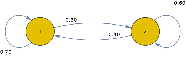
We will refer to the potential experts P_i, i.e. the probability functions in the frame, as the candidates.
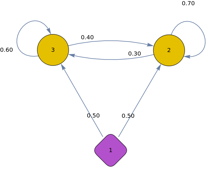
Notice that we can use this same structure to represent the full models of interest, where we have another function π, which may not be in the frame, and want to see whether π defers to the frame. The way to do so is just to treat world 1 as a “dummy world”, which gets assigned 0 probability by all worlds and which captures π’s credence function.
For example, the above frame combined with a π which is 50-50 between the two candidates, ca be represented as follows:
For example, the above frame combined with a π which is 50-50 between the two candidates, ca be represented as follows:
In[]:=
frame1plus={{0,0.5,0.5},{0,0.7,0.3},{0,0.4,0.6}}
Out[]=
{{0,0.5,0.5},{0,0.7,0.3},{0,0.4,0.6}}
In[]:=
MatrixForm[frame1plus]
Out[]//MatrixForm=
0 | 0.5 | 0.5 |
0 | 0.7 | 0.3 |
0 | 0.4 | 0.6 |
In[]:=
drawFrame[frame1plus]
Out[]=
In[]:=
This notebook contains special-made functions for generating, visualizing, and analyzing such frames. We will explain the functions in more detail in the sections below.
An example: we can generate a random 3-world frame:
An example: we can generate a random 3-world frame:
In[]:=
frame2=getRandFrame[3,7](*Thesecondargumentcontrolsthe"niceness"---howlargethedenominatorscanbe*)
Out[]=
,,,0,,,,,
4
15
1
15
2
3
1
2
1
2
1
5
2
25
18
25
We can visualize this by looking at the frame matrix:
In[]:=
MatrixForm[frame2]
Out[]//MatrixForm=
4 15 | 1 15 | 2 3 |
0 | 1 2 | 1 2 |
1 5 | 2 25 | 18 25 |
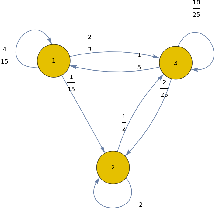
Or by looking at a Markov diagram of it:
In[]:=
drawFrame[frame2]
Out[]=
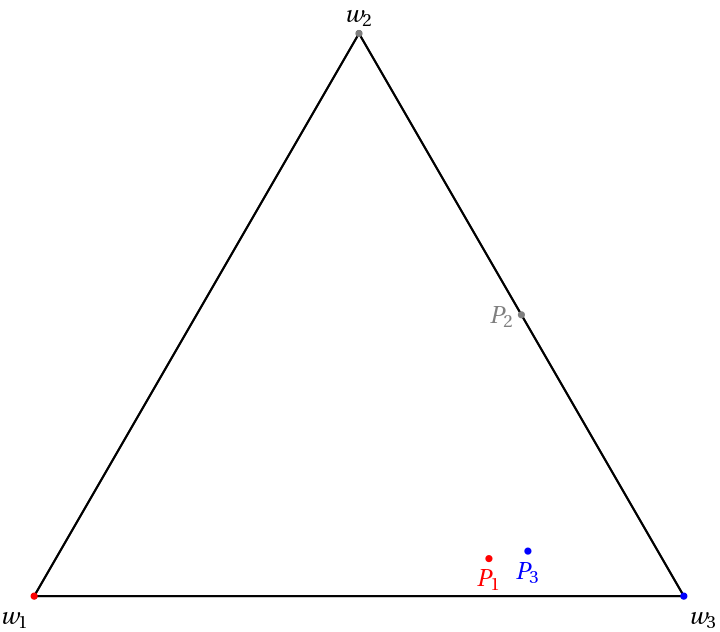
Or—by far the most helpfully—by visualizing it in a barycentric plot, in which the extreme points are the probability functions that are certain of each world, and the probability functions lie within this triangle (or, more generally, simplex):
In[]:=
plot3Frame[frame2,"none"]
Out[]=
And we can check whether it satisfies various properties. For instance, such as whether it validates Simple Trust, Trust, or Total Trust:
(A frame validates a constraint if all the functions P_i in the frame obey that constraint with respect to the frame.)
(A frame validates a constraint if all the functions P_i in the frame obey that constraint with respect to the frame.)
In[]:=
checkSimpleTrust[frame2]
Out[]=
False,x[1],x[2]-,x[3]-,t
4
5
1
5
1
5
1
5
In[]:=
checkTrust[frame2]
Out[]=
False,x[1]0,x[2],x[3]-,t
9
10
1
10
1
10
In[]:=
checkTotalTrust[frame2]
Out[]=
False,x[1]-1,x[2]-101,x[3]
21
2
Likewise for 4-world frames:
In[]:=
frame3=getRandFrame[4,8]
Out[]=
,,0,,,,,,,,,,,,,
3
28
9
28
4
7
5
22
7
66
29
66
5
22
7
66
1
6
4
11
4
11
6
17
12
85
21
85
22
85
In[]:=
MatrixForm[frame3]
Out[]//MatrixForm=
3 28 | 9 28 | 0 | 4 7 |
5 22 | 7 66 | 29 66 | 5 22 |
7 66 | 1 6 | 4 11 | 4 11 |
6 17 | 12 85 | 21 85 | 22 85 |
Such a process—especially finding frames with desired properties— can be computationally intensive. So this notebook also contains long lists of ready-made frames that have been checked to have certain properties. For example, it contains frames that validate Trust but not Total Trust (i.e. Value):
For example, we can see that world 3 of this frame is not modestly informed, since it falls outside the convex hull of it’s informed self (the blue dot in the corner of the simplex) and the other functions in the frame (you have to turn it to just the right angle to notice):
That gives a preview of what we’ll do; the rest of the notebook will explain the functions it contains, and give examples.
We break it into three sections: generating frames, visualizing frames, and analyzing frames.
NOTE: if you ever remember a function’s name, ‘FXN’, but can’t remember the inputs it requires, simply type ‘?FXN’ to receive the input (along with the code that runs it). For example:
We break it into three sections: generating frames, visualizing frames, and analyzing frames.
NOTE: if you ever remember a function’s name, ‘FXN’, but can’t remember the inputs it requires, simply type ‘?FXN’ to receive the input (along with the code that runs it). For example:
In addition, the final section contains a reference list of all functions used
Generating frames
Generating frames
In this section, we’ll describe the functions that go into generating probability frames, as well as the special class of them known as prior frames.
To generate a random probability frame with n worlds and a variance (amount of potential variation in probability fxn between worlds) v, use getRandFrame[n,v]:
This function simply uses the function getAnyRandProbVec[n,v] n different times, and collects them together:
Given a probability vector, we might want to check it’s various properties, such as the probability it assigns to some proposition q
We can also condition a probability vector, and then assess it’s conditional probabilities:
This function is useful for generating the subframes of a frame—namely, the set of frames you can get by conditioning all the worlds in the original frame on some proposition. (Notice, for example, that Trust is valid on a frame iff Simple Trust is valid on all of its subframes.)
To get the subframe resulting from conditioning on a single proposition q, use getOneSubFrame[frame,q]:
Now, often we want to generate a bunch of frames that have a particular property, as a way of randomly checking frames of that kind. For example, to test a conjecture that Total Trust entails some constraint C, it is useful to randomly generate a variety of Total-Trust frames, and then check whether each of them obeys C. If not, then you know that Total Trust does not entail that property; if so, then you get (defeasible) evidence that it does.
For example, one natural property of a frame is that it be p-reflexive, meaning that each world assigns more probability to itself than other worlds assign it: for all i,j: P_i(i) ≥ P_j(i).
Suppose we conjecture (falsely) that p-reflexivity entails Simple Trust. One way to check this is to pull a bunch of random frames, check whether they are p-reflexive, and if so gather them up. Then we run though the resulting list and see if Simple Trust is valid on all of them.
We have a function built in for checking p-reflexivity:
So we can use this to generate many p-reflexive frames:
This gives us a list of p-reflexive frames:
We can now check whether all of these validate Simple Trust, using the built-in function for that:
So we can see that the conjecture is false, since Simple Trust is not valid on all of these frames. (We’ll discuss more how to interpret this output below)
In fact, Simple Trust entails p-reflexivity (suppose P_i(j) ≥ t > P_j(j). Then P_i(j | P(j) ≥ t) = 0 < t.) As a result, sometimes we want to generate only p-reflexive frames. The following function (written by B.E.H.) allows us to do that efficiently. The syntax:
makePRefFrame[dim, maxIter, maxInt, seed], where
dim = the number of worlds
maxIter = the number of times the function attempts to construct a random p-reflexive frame of that size
maxInt = the “niceness” of the frame, controlling how finely the probabilities can vary
seed = an initial frame that can be used to work off of
We can also use this to generate a “n+1 frame”, with n worlds (n candidates for the expert) plus one probability function outside the frame (π), which we imagine deferring to it. Again, we model this by making the first world a “dummy world” that no world assigns positive probability to:
syntax: makePRefDimPlusFrame[n,niceness], where
n = number of worlds in frame, and
niceness = how much they can vary
syntax: makePRefDimPlusFrame[n,niceness], where
n = number of worlds in frame, and
niceness = how much they can vary
Prior frames, and trees
Prior frames, and trees
We can also generate a special subclass of probability frames known as prior frames (footnote 19 of the draft), in which there is a single (regular) prior, ρ, such that the probabilities at each world can be recovered by conditioning ρ on a particular proposition: ∀w ∈ W there is a R_w ⊆ W such that P_w(•) = ρ(•|R_w).
Such frames can be thought of as standard Kripke frames, wherein R_w is the set of worlds accessible from world w; it induces a binary relation R such that wRx iff x ∈ R_w.
In such a frame, the R_w are called the neighborhoods. We can generate such a frame by picking a prior and some neighborhoods over a fixed set of worlds:
Within prior frames, Value/Total Trust / Trust are each equivalent to the claim that the the neighborhoods form a tree (really, a “forest”): they are transitive (if x ∈ R_w, then R_x ⊆ R_w), shift-reflexive (if x ∈ R_w, then x ∈ R_x), and shift-nested (if x,y ∈ R_w, then either R_x ⊆ R_y or R_x ⊇ R_y or R_x ⋂ R_y = ∅). (Geanakoplos 1989, Theorem 1; Dorst 2020, Theorem 7.4)
We can efficiently generate very large such structures using a computational trick: the neighborhoods form a forest iff each world w can be associated with a sequence f(w) such that x ∈ R_w iff f(w) is an initial segment of f(x). (Dorst 2020, Theorem 5.8).
There are three functions involved in doing this. The first simply generates random neighborhoods for a given frame size, with two parameters to modulate the structure of the tree.
getRandTreeNbhds[frameSize, seqPoolSize, seqLength] , where
frameSize = the number of worlds in the frame
seqPoolSize = the size of the set of objects we are pulling random sequences from. The smaller the pool, the more likely it is that one world’s sequence will be an initial segment of another; the larger, the less likely this is.
seqLength = the max length of sequences we generate. This determines the maximum depth of the trees in the frame
The output of getRandTreeNbhds is several things. First, it gives you a sequence of {w, R_w} for each world w. Second, it assigns “nbd[w]” to R_w. This output is then used by the graphTree function to display the structure:
This function simply gives the structure of the prior frame; we need to add a prior in order to recover the probabilities at each world. The function
getRandTreeFrame[frameSize, seqPoolSize, seqLength]
uses the getRandTreeNbhds function, and then lays a regular prior over it to recover the probabilities at each world:
In doing so, it assigns frame” to the resulting probability frame this generates
getRandTreeFrame[frameSize, seqPoolSize, seqLength]
uses the getRandTreeNbhds function, and then lays a regular prior over it to recover the probabilities at each world:
In doing so, it assigns frame” to the resulting probability frame this generates
This function can be very useful for efficiently generating and checking properties of large validating frames—with the caveat that it only looks at the subset of them that are prior frames, of course.
Frame lists
Frame lists
Finally, since it can be computationally expensive to generate frames with various properties, this notebook comes pre-loaded with a variety “priorFrames” consists of a list of 100 randomly generated prior frames. None validate Trust or Total Trust
“priorTrees” consists of 100 randomly generated tree-shaped prior frames, which validate (Total) Trust
“noTrust” includes 48 frames that do not validate Trust but are p-reflexive
trustYesValueNo includes 4-world frames that validate Trust but not Total Trust / Value
TrustYesValueYes includes 4-world frames that validate both Trust and Total Trust/Value
totalTrustFrames includes more 4-world frames that validate total-Trust
totalTrust5Frames includes a few 5-world frames that validate Total Trust (these are computationally difficult to find—or at least they were before we knew that we could generate them using the modestly-informed constraint)
allValueProbFrames collects a large list of probability frames that validate Value / Total Trust
Finally, “pRefCondConvFrames” includes frames that are both p-reflexive and which are conditionally convex, which means that for each world i and proposition q, P_i(•|q) is in the convex hull of the P_j(•|q) such that j ∈ q. (This is a generalization of the “Reaction” constraint from Dorst 2020, §5.)
All of them validate Value; so we conjecture that p-reflexivity + conditional-convexity entails Value
All of them validate Value; so we conjecture that p-reflexivity + conditional-convexity entails Value
Visualizing Frames
Visualizing Frames
As we’ve seen with prior frames, certain frames are much easier to work with than others because they can be easily visualized. In our experience, this has been crucial for figuring out the constraints needed to validate certain principles.
Prior frames are easy to work with because they can be drawn simply as Kripke frames, with numbers assigned to worlds in order to recover their probabilities. That, for instance, is how I found that Trust was equivalent to the claim that the neighborhoods formed a tree---simply by drawing examples and checking whether they satisfied it.
In order to work with general probability frames, we need similar methods for visualizing them. The two simplest and most general are simply to draw them in stochastic-matrix of Markov-diagram notation:
matrix notation:
Markov diagram:
Unfortunately, these are not particularly illuminating to stare at. (Believe me, I’ve tried.)
The best method is to visualize them geometrically, treating each probability function as a vector in Euclidean n-space, for n the number of worlds, as discussed at length in DDB. Unfortunately, this only works up to a few dimensions; but it nevertheless makes it much easier to glob onto the necessary structures.
The best method is to visualize them geometrically, treating each probability function as a vector in Euclidean n-space, for n the number of worlds, as discussed at length in DDB. Unfortunately, this only works up to a few dimensions; but it nevertheless makes it much easier to glob onto the necessary structures.
Plotting 3-world frames
Plotting 3-world frames
We visualize this in a barycentric plot, which contains n extreme points, and each probability function over those n worlds is an average between them. In 3 dimensions this is a triangle. The command for plotting a 3-world frame is
plot3Frame[frame, cut], where
frame = the frame of interest, and
cut = the world i you wish to cut out to form the convex hull \hat{P_i} ⋃ {P_j: P_j≠P_i}, i.e. the set that P_i must fall within in order to be modestly informed. cut takes the values "none", 1, 2,...,n, or "all" do represent all such cuts at once.
Note that whenever each P_i is unique in the frame, then \hat{P_i} is simply the extreme point focused on world i. (Unfortunately, the way the "cut" system is written, it only works properly when each P_i is unique, since it always replaces P_i with it's world i)
Plot 3-world frames with (ignore the red “Delete”—it’s just how a piece of the code reacts to the “none” input)
As we can see, P_1 is modestly informed, since it lies inside the yellow convex hull:
Likewise (just barely) for P_2:
And P_3:
We can display them all together:
And indeed we can verify (more on this in the next section) that the frame validates Total Trust (and hence Value):
Suppose we alter the frame slightly by shifting P_3’s probability for P_2 slightly lower
We can see that P_3 now falls outside the relevant convex hull:
And, indeed, Total Trust now fails:
(It was looking at pairs of frames like this and checking each for Total Trust, by the way, which allowed us to cotton on to the characterization in terms of modest-informedness.)
To manipulate a frame by hand, you can use the visualize3Frame function (don’t worry about the red):
(NOTE: sometimes—I’m not sure why—this visualization starts constantly recomputing without any input, which can slow your machine down. wrap the below command in (* *) and execute it to stop this, i.e. write
(* visualize3Frame *)
then hit shift + enter
(NOTE: sometimes—I’m not sure why—this visualization starts constantly recomputing without any input, which can slow your machine down. wrap the below command in (* *) and execute it to stop this, i.e. write
(* visualize3Frame *)
then hit shift + enter
This function displays a variety of things, with a variety of options. The sliders allow you to control the probabilities at each world. ‘w1’ is how self-confident P_1 is, i.e. P_1(1). ‘w1b’ is the balance P_1 gives between worlds 2 and 3, so w1b = P_1(2|2 or 3). Similarly, w2 is P_2(2), and w2b is P_2(1| 1 or 3); and w3 is P_3(3) and w3b is P_3(1| 1 or 2). By sliding these around, you can move the functions around the triangle (try it!)
(Confusing things:
– the color code is red = P_1, gray = P_2, blue = P_3
– unlike our other diagrams, w1 is in the bottom right, w2 is in the bottom left, and w3 is in the top. (One day I’ll get around to fixing this...))
– the color code is red = P_1, gray = P_2, blue = P_3
– unlike our other diagrams, w1 is in the bottom right, w2 is in the bottom left, and w3 is in the top. (One day I’ll get around to fixing this...))
The purple dot is the stationary distribution of the frame, i.e. the (unique) probability function ρ such that, where F is the frame matrix, ρF = ρ. Equivalently, ρ expectation-matches the frame, meaning that for all q: ρ(q) = _ρ(P(q)), where ‘P’ is a definite description for the expert probability function. Raising the matrix F to higher and higher powers leads each of the functions in it to converge to this stationary (this is the Markov chain convergence theorem; a consequence of the Perron-Frobenius theorem). The “power” function allow you to see this convergence in steps, with orange dots that move toward the purple one. We’ll talk a bit more about stationaries later.
Finally, the row with the “no lines” option, and the “delete” row allow you to look at various subframes of the frame, i.e. the result of conditioning all the functions in the frame on a given proposition. Conditioning them on ¬{1} projects each function through the line between it and the extreme point 1, for instance.
Once you do this, you may notice that the purple and orange dots come apart. The purple is the result of conditioning the original stationary distribution on the proposition in question. The orange dot is the result of first conditioning every world in the frame on that proposition, and then taking their stationary. The fact that these can come apart is both formally and perhaps philosophically interesting—Daniel Rothschild has some cool results about this.
3+-frames and 4-frames
3+-frames and 4-frames
Okay enough of that rabbit hole. Final things to show with visualization:
As demonstrated at the beginning, we can visualize a 3+1 frame which has an extra probability function over it:
As demonstrated at the beginning, we can visualize a 3+1 frame which has an extra probability function over it:
We can visualize 4-world frames using a 3D barycentric plot
(color-code:
red = w1 and P_1,
gray = w2 and P_2
blue = w3 and P_3
orange = w4 and P_4
(color-code:
red = w1 and P_1,
gray = w2 and P_2
blue = w3 and P_3
orange = w4 and P_4
For example here is a modestly-informed 4-frame:
Higher dimensions
Higher dimensions
Obviously there are hard limits on how much we can visualize in higher dimensions. But one strategy is to take various subframes of a higher-dimensional frame to see the “shadow” it casts in lower dimensions.
So, for instance, we can take a 5-world Total Trust frame, and look at all the 4-world subframes it generates—i.e. those obtained by conditioning on the negation of a given world thus projecting away from that world in the 4D simplex that covers this frame’s barycentric plot
So, for instance, we can take a 5-world Total Trust frame, and look at all the 4-world subframes it generates—i.e. those obtained by conditioning on the negation of a given world thus projecting away from that world in the 4D simplex that covers this frame’s barycentric plot
(Unfortunately, this doesn’t (yet) have the functionality to plot the probabilities of the world that has been ruled out, so e.g. in the first shadow we’ve plotted P_2(•|¬{1}), P_3(•|¬{1}), etc., but not P_1(•|¬{1}))
Analyzing frames
Analyzing frames
Suppose we’ve generated and/or visualized some frames. In order to draw useful from conclusions from this, we need functions that can efficiently what properties they have. If you’re exploring the constraints imposed by a given deference principle, the best strategy is to write a custom “frame checker” for that principle, and then to generate many frames and see what the ones that validate that principle have in common.
An in-depth example:
An in-depth example:
To illustrate the methodology, we’ll illustrate how we discovered the modestly-informed characterization of Total Trust. First, we make a function that can check a frame for whether it validates Total Trust:
Here’s the code for the function; the way it works is as follows. (Skip this if you don’t care about the details.) For Total Trust , for any random variable X:
E_π(X | E(X) ≥ t) ≥ t.
Noting that X-t is also a random variable, this is equivalent to: for any random variable Y,
E_π(Y | E(Y) ≥ 0 ) ≥ 0.
As explained in the paper, this can hold for some π iff it holds for each world in the frame, i.e. where E_i is world i’s expectation function, we have that for all i and random variables Y,
E_i(Y | E(Y)≥0) ≥ 0.
Given a frame, the function generates an algebraic expression which says what it would mean for this to fail for an arbitrary Y, and then calls Mathematica’s (very powerful, but very computationally expensive) “FindInstance” function to see if it can find a random variable that meets those constraints. If it finds such, it gives the relevant random variable; if it establishes that there is no such variable, it says that Total Trust is valid.
In detail:
We can then generate a variety of frames, and sort them into those that did and did not validate total trust, for example with code like the following: (this takes about a minute to run on my machine):
We can then generate a variety of frames, and sort them into those that did and did not validate total trust, for example with code like the following: (this takes about a minute to run on my machine):
We can then try to notice differences between the two sets of frames by visualizing them
Staring at these frames, we can see that the former are modestly informed and the latter are not
Once we form a conjecture like this, we can make a checker for the relevant property (modest-informedness), and see whether this matches the verdicts for Total Trust across all examples we have. The following function checks that:
Once we get results like these, we can go about looking for an analytic proof
Summary of checkers
Summary of checkers
This subsection summarizes the checkers built in to the above functions. All of them check whether the principle is valid on the frame, i.e. whether for all probability functions P_i in the frame, they obey the relevant constraint.
Total Trust/Value: E_i(X | E(X)≥t) ≥ t, for all X,t, for all worlds i
If false, the output gives you the random variable on which it fails. Using this, you can check where exactly it fails by making the relevant assignments:
This tells us that the only world with non-negative expectation for X is world 1, yet the value of X at world 1 is -1. Thus, for example, E_1(X | E(X)≥0) = –1, and total Trust fails.
Trust: P_i(q | p& P(q|p) ≥ t ) ≥ t for all q, p, t.
This function has strange output, due to the fact that it piggybacks off the checkTotalTrust function. Read it as follows. x[i] is set to 0 iff i ∉ p, x[i] > 0 if i ∈ q; the negative assignments are for those i that are not in q but are in p.
So we can read this example as saying that Trust fails for some world with the instance q = {2}, p = {2,3}, and t = 2/5.
So we can read this example as saying that Trust fails for some world with the instance q = {2}, p = {2,3}, and t = 2/5.
Simple Trust: P_i(q | P(q) ≥ t) ≥ t for all q, t
Read this like the output for the checkTrust checker, only no assignments will be 0 since there is no option to condition on some event
Simple Reliance (Dorst 2020, EAGU): P_i(q | P(q) ≥ t) ≥ P_i(q)
Here let q = {4} and t = 11/30
Reliance (Dorst 2020, EAGU): P_i(q | p& P(q|p) ≥ t) ≥ P_i(q|p)
Honestly, I don’t remember how to read this output. Take it with a grain of salt X).
Conditional Convexity: for any q, P_i(•|q) is in the convex hull of the P_j(•|q) such that P_i(j|q) > 0, i.e. conditional on q, you’re in the convex hull of the candidate experts you leave open given that. (This is a generlization of the “Reaction” principle from Dorst 2020, EAGU, used to characterize Trust. It entails, but is not entailed by, New Reflection.)
The failures output tells you what to condition on ({1,2,4}), and which world fails the constraint when so conditioned (3).
New Reflection: P_i(• | P = ρ) = ρ(• | P=ρ)
p-reflexivity: for all i,j: P_i(i) ≥ P_j(i)
Reflexivity: for all i, P_i(i)>0
Shift-Reflexivity: for all i, if there is a j such that P_j(i)>0, then P_i(i)>0
Transitivity: for all i,j,k, if P_i(j)>- and P_j(k)>0, then P_i(k)>0
Shift-Nested: if i,j ∈ R_k, then either R_i ⊆ R_j or R_i ⊇ R_j or R_i ⋂ R_j = ∅
Tree: is shift-reflexive, shift-nested, and transitive
Propositional p-reflexivity: for all propositions q, if i ∈ q and j ∉ q, the P_i(q) ≥ P_j(q)
(This is a strong constraint, not entailed by Value, but also not trivializing)
(This is a strong constraint, not entailed by Value, but also not trivializing)
Glossary of functions
Glossary of functions
Generating frames, and manipulation utilities
Generating frames, and manipulation utilities
getAnyRandProbVec[x, y] generates a random probability vector of x worlds with y a parameter for how much the world probabilities can vary
getRegProbVec[x,y] generates a random regular probability vector over x worlds with y a parameter for how much the world probabilities can vary
probability[vec, prop] gives the probability that the probability vector vec assigns to the proposition prop
condition[vec,prop] conditions the probability vector vec on the proposition prop
getRandFrame[n,var] generates a random frame of n worlds with var a parameter for how much the world probabilities can vary
getSubFrames[frame] generates a list of all the subframes of frame
makePRefFRame[n, x , var, seed] generates a random p-reflexive frame of n worlds (with x attempts—set it to 1000), with variance var, using seed as a frame to work off of (can input None)
makePRefDimPlusFrame[n,var] generates a random n+-world frame, i.e. one in which world 1 is a dummy world seen by nothing, treated just as an extra probability distribution over the n remaining worlds
getRandNbds[n] generates random neighborhoods for a size n frame
getFrame[p, nbds] generates a prior frame using the prior p and the neighborhoods nbds.
getRandTreeNbhds[n, x, y] generates a random tree-shaped neighborhoods over n worlds with x and y parameters controlling the possible width and height of the tree
getRandTreeFrame[n,x,y] does the same, but also generates a random prior of n worlds and uses it to generate the full frame using the neighborhoods
Visualizing frames
Visualizing frames
graphtree can be used after getRandTreeNbhds or getRandTreeFrame to display the structure of the tree
drawFrame[F] draws the markov diagram of the frame F
MatrixForm[F] puts the frame in stochastic matrix form
visualize3Frame generates a manipulable object where you can move the probabilities in a given 3-world frame around manually
plot3Frame[F,c] displays the 3-world frame F in a barycentric plot. c can take the values “none”, 1, 2,3, or “all”, and it says which modest-informed convex hulls to display
plot3PlusFrame[F,c] takes a 3+ frame, i.e. a 4-row square matrix where the first column is all 0s (so the first world is a dummy world), and plots both the 3-world frame and the extra probability distribution over it. c plays the same function as above.
plot4Frame[F,c] displays the 4-world frame F in a barycentric plot. c can take on the values “none”, 1, 2, 3, 4, “all”.
Checking frame conditions
Checking frame conditions
isRef[F] checks whether F is reflexive: for all i, P_i(i)>0
isShiftRef[F] checks whether F is shift-reflexive: for all i,j: if P_j(i)>0, then P_i(i)>0
isPRef[F] checks whether F is p-reflexive: for all i,j: P_i(i) ≥ P_j(i)
isTrans[F] checks whether F is transitive: for all i, j, k: if P_i(j)>0 and P_j(k)>0 then P_i(k)>0
isShiftNested[F] checks whether F is shift-nested: for all i, j, k: if i,j ∈ R_k, then either R_i ⊆ R_j or R_j ⊇ R_i or R_i ⋂ R_j = ∅
isTree[F] checks whether F is a tree, i.e. whether it is shift-reflexive, transitive, and shift-nested
checkPropPRef[F] checks whether F is propositionally reflexive: if i ∈ q and j ∉ q, then P_i(q) ≥ P_j(q)
checkPropPRefCase[F,prop] yields the minimum P_i(q) such that i ∈ prop and max P_j(q) such that j ∉ prop
checkSimpleTrust[F] checks whether Simple Trust is valid on F: P_i(q | P(q) ≥ t) ≥ t
checkTrust[F] checks whether Trust is valid on F: P_i(q | p & P(q|p)≥t) ≥ t
inConvexHull[F, π] checks whether the probability vector π is in the convex hull of the frame F
checkCondConv[F] checks whether the F is conditionally convex: if P_i(•|q) is in the convex hull of the P_j(•|q) such that j ∈ q
checkSimpleReliance[F] checks whether Simple Reliance is valid on F: P_i(q | P(q) ≥ t) ≥ t
checkFullReliance[F] checks whether Reliance is valid on F: P_i(q | p & P(q|p) ≥ t) ≥ P(q|p)
checkEReliance[F] checks whether E-Reliance is valid on F: for any random variable X, E_i(X | E(X) ≥ t) ≥ E_i(X). (Total Trust entails E-Reliance; the converse may for all we know be true.)
checkRP[F] checks whether the ratio-preservation strengthening of Trust is valid: for all p, q, and number t: P_i(q | P(q) ≥ t*P(p) ) ≥ t*P(p | P(q) ≥ t * P(p)). (ratio-preservation is entailed by Total Trust, entails Trust, and is not entailed by Trust.)
checkTotalTrust[F] checks whether Total Trust is valid on F: E_i(X | E(X) ≥ t) ≥ t
checkNR[F] checks whether New Reflection is valid on F: P_i ( • | P = ρ) = ρ(• | P = ρ)