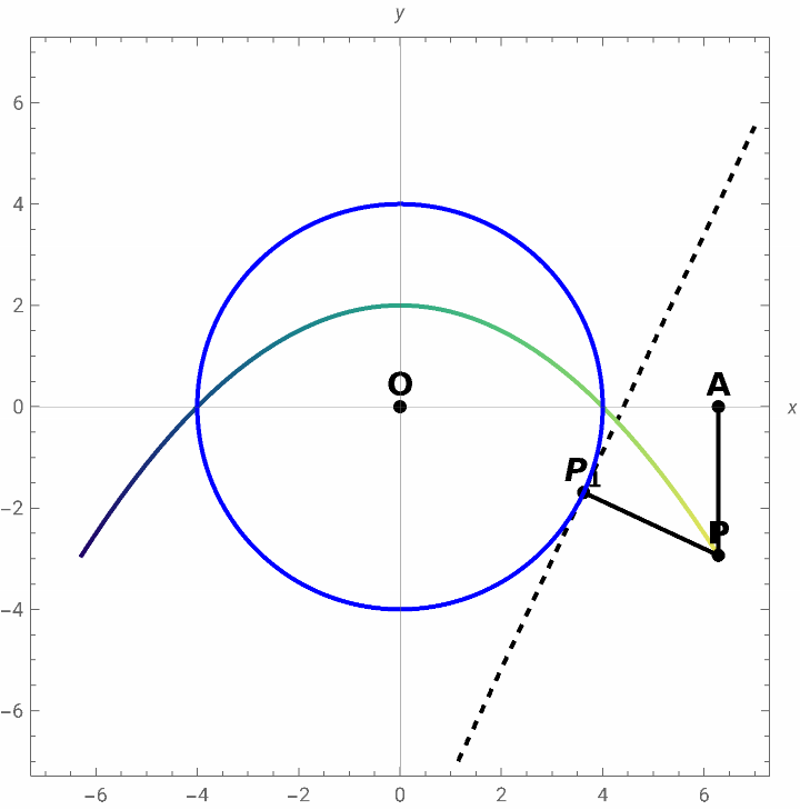
Development:
Let P be of coordinates (x, y) and be the point of contact between the normal and the tangent to the circumference then according to the figure and by the Pythagorean theorem, it is fulfilled that:
P
1
2
x
2
y
2
+r
PP
1
Then,based on the geometric locus described we know that = y, then:
PP
1
2
x
2
y
2
(y+r)
Solving for y , the answer remains:
±y=+-r
2
x
2
y
Doing operations there are 2 equations left:
2
x
r
2
2
x
r
2
In[]:=
Manipulater=4;P1[x_]:=,4-16;P[x_]:=x,;O1={0,0};A1[x_]:={x,0};d1=Norm[P[x1]-P1[x1]];d2=Norm[P[x1]-A1[x1]];t=Grid[{{,},{N[d1],N[d2]}},FrameAll,ItemStyle->15,ItemSize15];ShowContourPloty-4-16==-x-,{x,-7,7},{y,-7,7},ContourStyle{Black,Dashed},ParametricPlot[P[x],{x,-2π,x1},ColorFunction->"BlueGreenYellow"],Graphics[{Black,PointSize[0.018],Point[O1],Text[Style["O",14,Bold],O1,{0,-1.2}],Point[P[x1]],Text[Style["P",14,Bold],P[x1],{0,-1.2}],Point[P1[x1]],Text[Style["",14,Bold],P1[x1],{0,-1.2}],Point[A1[x1]],Text[Style["A",14,Bold],A1[x1],{0,-1.2}],Thick,Line[{P[x1],A1[x1]}],Line[{P[x1],P1[x1]}],Blue,Thick,Circle[O1,r]}],AspectRatioAutomatic,AxesTrue,AxesOrigin{0,0},AxesLabel{x,y},PlotRange7,Style["Case 1 parabola",Bold,Large],{{x1,-2π+0.00002,"Value ()"},-2π+0.000001,2π,0.00001},Delimiter,{{t,3,"Distance from point P to circumference () and from point P to point A "}},ControlPlacementTop
32x1
256+32+
2
x1
4
x1
2
x1
16+
2
x1
-+
2
r
2
x
2r
PP
1
PA
2
x1
16+
2
x1
2rx1
2
r
2
x1
32x1
256+32+
2
x1
4
x1
P
1
x
1
P
1
Out[]=


In[]:=
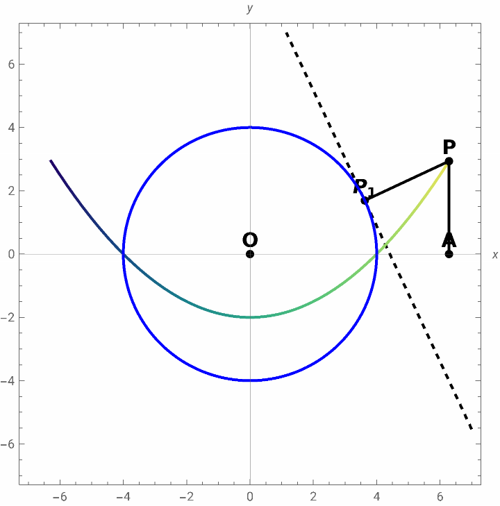
Manipulater=4;P1[x_]:=,4;P[x_]:=x,-;O1={0,0};A1[x_]:={x,0};d1=Norm[P[x1]-P1[x1]];d2=Norm[P[x1]-A1[x1]];t=Grid[{{,},{N[d1],N[d2]}},FrameAll,ItemStyle->15,ItemSize15];ShowContourPloty-4==-x-,{x,-7,7},{y,-7,7},ContourStyle{Black,Dashed},ParametricPlot[P[x],{x,-2π,x1},ColorFunction->"BlueGreenYellow"],Graphics[{Black,PointSize[0.018],Point[O1],Text[Style["O",14,Bold],O1,{0,-1.2}],Point[P[x1]],Text[Style["P",14,Bold],P[x1],{0,-1.2}],Point[P1[x1]],Text[Style["",14,Bold],P1[x1],{0,-1.2}],Point[A1[x1]],Text[Style["A",14,Bold],A1[x1],{0,-1.2}],Thick,Line[{P[x1],A1[x1]}],Line[{P[x1],P1[x1]}],Blue,Thick,Circle[O1,r]}],AspectRatioAutomatic,AxesTrue,AxesOrigin{0,0},AxesLabel{x,y},PlotRange7,Style["Case 2 parabola",Bold,Large],{{x1,-2π+0.00002,"Value ()"},-2π+0.000001,2π,0.00001},Delimiter,{{t,3,"Distance from point P to circumference () and from point P to point A "}},ControlPlacementTop
32x1
256+32+
2
x1
4
x1
16-
2
x1
16+
2
x1
2
r
2
x
2r
PP
1
PA
16-
2
x1
16+
2
x1
2rx1
2
x1
2
r
32x1
256+32+
2
x1
4
x1
P
1
x
1
P
1
Out[]=