Boundary Layer in Flow between Parallel Plates
Boundary Layer in Flow between Parallel Plates


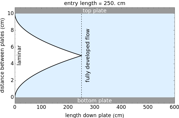
This Demonstration calculates the thickness of a boundary layer for flow between stationary parallel plates as a function of distance down the plates. You can vary the distance between the plates, fluid velocity and kinematic viscosity with sliders. The boundary layer (shaded light blue region) represents the region where viscous forces must be taken into account due to the no-slip condition. Outside of the boundary layer (white region), viscous forces are negligible. Once the two boundary layers meet midway between the plates, the fluid flow is fully developed.
Details
Details
The Prandtl–Blasius boundary layer solution is used:
δ
L
5x
1/2
Re
δ
T
0.37x
1/5
Re
Re=
ux
ν
where and are boundary layer thickness for laminar and turbulent flow (cm), is length down the plates (cm), is the Reynolds number (dimensionless), is fluid velocity (cm/s) and is kinematic viscosity (/s).
δ
L
δ
T
x
Re
u
ν
2
cm
Fluid flow is laminar for and turbulent for . The boundary layer thickness for the transition region () is calculated from:
Re<2×
5
10
Re>3×
6
10
δ
R
2×≤Re≤3×
5
10
6
10
δ
R
δ
L
δ
T
f=-
x-
x
L
x
T
x
L
x
L
5
10
ν
u
x
T
6
10
ν
u
where is the fraction of flow in the transitions region that is turbulent, and and are the boundaries of the laminar and turbulent regions (cm).
f
x
L
x
T
References
References
[1] B. R. Munson, T. H. Okiishi, and W. W. Huebsch, Fundamentals of Fluid Mechanics, 6th ed., Hoboken, NJ: John Wiley & Sons, 2010.
Permanent Citation
Permanent Citation
Jaeda C. Sichel, Rachael L. Baumann, Garret D. Nicodemus
"Boundary Layer in Flow between Parallel Plates"
http://demonstrations.wolfram.com/BoundaryLayerInFlowBetweenParallelPlates/
Wolfram Demonstrations Project
Published: April 28, 2014