ABSTRACT (original article): In 1914, Ramanujan presented 17 infinite series for . We examine the physics origin of these remarkable formulae by connecting them to 2D logarithmic conformal field theories (LCFTs) which arise in various contexts such as the fractional quantum hall effect, percolation and polymers. In light of the LCFT connection, we investigate such infinite series in terms of the physics data, i.e., the operator spectrum and OPE coefficients of the CFT and the conformal block expansion. These considerations lead to novel approximations for . The rapid convergence of the Ramanujan series motivates us to take advantage of the crossing symmetry of the LCFT correlators to find new and efficient representations. To achieve this, we use the parametric crossing symmetric dispersion relation which was recently developed for string amplitudes. Quite strikingly, we find remarkable simplifications in the new representations, where, in the Legendre relation, the entire contribution to comes from the logarithmic identity operator, hinting at a universal property of LCFTs. Additionally, the dispersive representation gives us a new handle on the double-lightcone limit. CITATION (original article): Faizan Bhat, Aninda Sinha (2025), Logging the conformal life of Ramanujan’s π, arXiv:2503.21656. https://doi.org/10.48550/arXiv.2503.21656
1/π
1/π
1/π
From the Legendre Relation to Ramanujan’s 1/π formulae via Modular Equations
From the Legendre Relation to Ramanujan’s 1/π formulae via Modular Equations
In[]:=
Quit[];
In[]:=
$MaxExtraPrecision=500;
The Legendre Relation is given as follows (Equation 3)
The Legendre Relation is given as follows (Equation 3)
In[]:=
F[z_,σ_]:=Hypergeometric2F1[σ,1-σ,1,z];
In[]:=
FF1[z_,zbar_,σ_]:=F[z,σ]F[1-zbar,σ];
In[]:=
LegReln[Z_,σ_]:=(z(1-z)D[FF1[z,zbar,σ],z]-zbar(1-zbar)D[FF1[z,zbar,σ],zbar])/.z->Z/.zbar->Z//FullSimplify;
1
Sin[πσ]
Mathematica is able to simplify the expression for z = 1/2 but not for z ≠ 1/2. So we verify the expressions numerically there
In[]:=
{LegReln[1/2,1/2],LegReln[1/2,1/3],LegReln[1/2,1/6]}
Out[]=
,,
1
π
1
π
1
π
In[]:=
Table[LegReln[zz,ss]/.{zz->RandomReal[{0,1}],ss->RandomReal[{0,1}]},{n,1,100}]
Out[]=
{0.31831,0.31831,0.31831,0.31831,0.31831,0.31831,0.31831,0.31831,0.31831,0.31831,0.31831,0.31831,0.31831,0.31831,0.31831,0.31831,0.31831,0.31831,0.31831,0.31831,0.31831,0.31831,0.31831,0.31831,0.31831,0.31831,0.31831,0.31831,0.31831,0.31831,0.31831,0.31831,0.31831,0.31831,0.31831,0.31831,0.31831,0.31831,0.31831,0.31831,0.31831,0.31831,0.31831,0.31831,0.31831,0.31831,0.31831,0.31831,0.31831,0.31831,0.31831,0.31831,0.31831,0.31831,0.31831,0.31831,0.31831,0.31831,0.31831,0.31831,0.31831,0.31831,0.31831,0.31831,0.31831,0.31831,0.31831,0.31831,0.31831,0.31831,0.31831,0.31831,0.31831,0.31831,0.31831,0.31831,0.31831,0.31831,0.31831,0.31831,0.31831,0.31831,0.31831,0.31831,0.31831,0.31831,0.31831,0.31831,0.31831,0.31831,0.31831,0.31831,0.31831,0.31831,0.31831,0.31831,0.31831,0.31831,0.31831,0.31831}
Final form of the Legendre relation
Final form of the Legendre relation
Now we use the modular equations to bring the Legendre relation to the final form (Equation 11) where we use the Clausen identity to replace witha3F2 Hypergeometric function
2
F[z,σ]
In[]:=
LegRelnMod[σ_,n_]:=z0[n](1-z0[n])DHypergeometricPFQσ,1-σ,,{1,1},4Z(1-Z),Z/.Z->z0[n]+α[n]HypergeometricPFQσ,1-σ,,{1,1},4z0[n](1-z0[n]);
1
Sin[πσ]
1/2
n
1
2
1
2
lets check this for , , which leads to the Ramanujan’ s formula given in Equation 12
σ=1/2
n=3
1/π
In[]:=
z0[3]=2-;
1
4
3
;α[3]=4
3
In[]:=
N[LegRelnMod[1/2,3],{∞,10}]
Out[]=
0.318309886
We can now write down the Modular Legendre Relations at larger n as well
In[]:=
z0[1]=;α[1]=0;z0[2]=3-22+2-;z0[7]=8-3;z0[12]=49-20+54+68;z0[64]=;α[64]=-;z0[58]=;α[58]=+++;z0[1024]:=;α[1024]:=+32-1-+3+6+6+2-321-;
1
2
2
;α[2]=1
4
2
;z0[3]=1
4
3
;α[3]=4
3
1
16
7
;α[7]=80
7
4
-1+
2
6
;α[12]=153
2
2
+11577
6
2
4
-1+
2
1/4
-4+3
2
4
1+
2
1/4
-4+3
2
4
1+
2
1/4
-4+3
2
8-5+4-2
1/4
2
2
+43/4
2
4
+
5/8
2
1+
2
8
4
-1+
2
1/4
(-4+3
2
)4
1+
2
1/4
(-4+3
2
)81-
4
-1+
2
1/4
-4+3
2
4
-1+
2
1/4
(-4+3
2
)4
1+
2
1/4
(-4+3
2
)1
384238403+71351280
29
+19823765920568201+699313893460
29
32119361
2
22712397
2
86484024
29
244607523
2
58
4
-1+
1/4
1-
4
-1+
2
1/4
(-4+3
2
)4
1+
2
1/4
(-4+3
2
)4
1+
1/4
1-
4
-1+
2
1/4
(-4+3
2
)4
1+
2
1/4
(-4+3
2
)4
1+
1/4
1-
4
-1+
2
1/4
-4+3
2
4
1+
2
1/4
-4+3
2
128-7+4
2
+4-4+3
2
4
1++
2
1/4
-4+3
2
7/8
2
1/4
+2
1/4
-4+3
2
3/4
-4+3
2
2
1/4
-4+3
2
7/8
2
1/4
+2
1/4
-4+3
2
3/4
-4+3
2
2
1/4
-4+3
2
-4+3
+22
3/4
2
1/4
-4+3
2
3/4
-4+3
2
3
1++
2
1/4
-4+3
2
7/8
2
1/16
-4+3
2
1/4
1+2
-4+3
2
32
4
-1+
1/4
1-
4
-1+
2
1/4
(-4+3
2
)4
1+
2
1/4
(-4+3
2
)4
1+
1/4
1-
4
-1+
2
1/4
(-4+3
2
)4
1+
2
1/4
(-4+3
2
)4
-1+
1/4
1-
4
-1+
2
1/4
-4+3
2
4
1+
2
1/4
-4+3
2
4
-1+
1/4
1-
4
-1+
2
1/4
(-4+3
2
)4
1+
2
1/4
(-4+3
2
)4
1+
1/4
1-
4
-1+
2
1/4
(-4+3
2
)4
1+
2
1/4
(-4+3
2
)In[]:=
N[{LegRelnMod[1/2,7],LegRelnMod[1/2,12],LegRelnMod[1/2,58],LegRelnMod[1/2,64],LegRelnMod[1/2,1024]},{∞,10}]
Out[]=
{0.318309886,0.318309886,0.318309886,0.318309886,0.318309886}
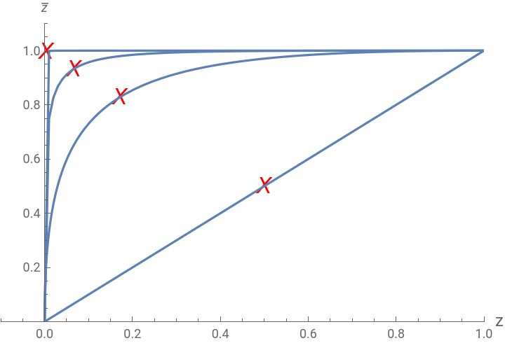
Modular conditions and singular values for n =1,2,3,4. This leads to Figure 1
Modular conditions and singular values for n =1,2,3,4. This leads to Figure 1
Plot[z,{z,0,1},PlotRange{0,1}];Plot[4Sqrt[z]/(1+Sqrt[z])^2,{z,0,1},PlotRange->{0,1}];ListPlot[Prepend[Append[Table[{z,(zb/.NSolve[(zzb)^(1/4)+(1-z)^(1/4)(1-zb)^(1/4)==1,zb,Reals,30][[2]])},{z,0.01,1-0.01,0.01}],{1,1}],{0,0}],JoinedTrue];ListPlot[Prepend[Append[Table[{z,(zb/.NSolve[(zzb)^(1/8)+(1-z)^(1/8)(1-zb)^(1/8)==1,zb,Reals,30][[2]])},{z,0.01,1-0.01,0.01}],{1,1}],{0,0}],JoinedTrue];ListPlot[{{1/2,1/2},{3-2Sqrt[2],1-(3-2Sqrt[2])},{(2-Sqrt[3])/4,1-(2-Sqrt[3])/4},{((3-Sqrt[7])/(4Sqrt[2]))^2,1-((3-Sqrt[7])/(4Sqrt[2]))^2}},PlotRange->{{-0.1,1},{0,1.1}},PlotMarkers{"X"},PlotStyle->{Red,Thick}];Show[{%,%%,%%%,%%%%,%%%%%},AxesLabel->{"z",OverBar[z]},ImageSize->Large]
Out[]=
Usual Conformal Block Expansion for Log CFTs and new formulae for 1/π
Usual Conformal Block Expansion for Log CFTs and new formulae for 1/π
2D Global Blocks and the Log part of the correlator as in Eq. 19 and Eq. 20
In[]:=
FFLog[z_,zbar_,σ_]:=-F[z,σ]F[zbar,σ];
Sin[πσ]
π
In[]:=
kfunc[β_,x_]:=Hypergeometric2F1,,β,x;Block2DZ[z_,zbar_,DD_,l_]:=kfunc[DD+l,z]kfunc[DD-l,zbar]+kfunc[DD-l,z]kfunc[DD+l,zbar];
β/2
x
β
2
β
2
Extracting OPE Coefficients
Extracting OPE Coefficients
In[]:=
zmax=zbmax=6;lmax=6;nmax=6;FFLogBlockExp=SeriesSumC2[2n+l,l,σ]Block2DZ[z,zbar,2n+l,l],{l,0,lmax},{n,0,nmax},{z,0,zmax},{zbar,0,zbmax}//PowerExpand//Simplify//Normal;FFLogBlockExpCoeff[zp_,zbp_]:=SeriesCoefficient[FFLogBlockExp,{z,0,zp},{zbar,0,zbp}];FFLogExp=Series[FFLog[z,zbar,σ],{z,0,zmax},{zbar,0,zbmax}]//Normal;FFLogExpCoeff[zp_,zbp_]:=SeriesCoefficient[FFLogExp,{z,0,zp},{zbar,0,zbp}];Solve[And@@DeleteCases[Flatten[Table[FFLogBlockExpCoeff[zp,zbp]==FFLogExpCoeff[zp,zbp],{zp,0,zmax},{zbp,0,zbmax}],1],True],Flatten[Table[C2[2n+l,l,σ],{l,0,lmax},{n,0,nmax}]]]//SimplifyClear[zmax,zbmax,lmax,nmax,σ]
-(1-σ)σ
((1-z)(1-zbar))
-Sin[πσ]
π
1
2
Ramanujan’s 1/pi (Legendre Relation) in terms of Conformal Data (Equation 21)
Ramanujan’s 1/pi (Legendre Relation) in terms of Conformal Data (Equation 21)
We write the block decomposition of the Log Part of the correlator as in Equation 20
When plugged in to the Legendre Relation, we get the conformal block expansion of 1/π
Approximation to 1/π from conformal data as given in equation 21
This gives 6 decimal places agreement with 1/π as we see numerically
Faster converging Conformal Block Expansions for 1/π using Modular Equations
Faster converging Conformal Block Expansions for 1/π using Modular Equations
We restrict to σ = 1/2; z0[n] and α[n] were defined before. We get more and more decimal place agreement as we increase the order of the modular equation. This exercise leads to the Table 1 in the Supplementary material
With only identity operator
With all operators upto nmax = lmax = 6
Simple approximations for 1/π as given in Equation 28 and 29
Simple approximations for 1/π as given in Equation 28 and 29
Parametric, Crossing Symmetric Dispersion Relations and Universality in Log CFTs
Parametric, Crossing Symmetric Dispersion Relations and Universality in Log CFTs
We express the left/right correlator using the Parametric, Crossing Symmetric Dispersion Relation (PCSDR) as in Equation 24
Lets check this expression and verify that its λ independent
Now we express the Legendre relation using PCSDR
Now we express the Legendre relation using PCSDR
Lets check this expression and verify that its λ independent
New dispersive block expansion
New dispersive block expansion
Now we can plug in the conformal block decomposition of the FFLog term in the dispersive representation above to get a new dispersive block expansion. We compare it with the usual block decomposition to show that it converges faster. This leads to the heat plots in Figure 2.
In the large λ limit, the log-identity operator gives the entire contribution in the Legendre Relation
In the large λ limit, the log-identity operator gives the entire contribution in the Legendre Relation
We then use the dispersive block expansion in the Legendre relation. We show that in the large λ limit, the log-identity operator gives the entire contribution in the Legendre Relation. This universality property is demonstrated by Figure 3.
Lets check this representation and verify that convergence improves as λ is increased . We will stick to nmax = 2; lmax = 2;
Log - Identity operator gives the full contribution in the large λ limit
CITE THIS NOTEBOOK
CITE THIS NOTEBOOK
Logging the conformal life of Ramanujan's π
by Faizan Bhat, Aninda Sinha
Wolfram Community, STAFF PICKS, April 2, 2025
https://community.wolfram.com/groups/-/m/t/3438221
by Faizan Bhat, Aninda Sinha
Wolfram Community, STAFF PICKS, April 2, 2025
https://community.wolfram.com/groups/-/m/t/3438221