As a follow-on to my earlier post about Epidemiological Models for Influenza and COVID-19, I’d like to show how these compartmental models can be used in a stochastic setting to study how the inherent randomness of events can affect the interpretation of modeled outcomes.
As noted before, the deterministic ODE-based models have a number of assumptions:
◼
All of the individuals of a given type are identical
◼
The population of individuals is well mixed, that is, instantaneously and uniformly mixed
◼
The number of individuals is so large that the density can be treated as a continuous variable
The last assumption rarely holds in practice for epidemiology models where the number of individuals is typically on the order of hundreds to millions. These population sizes are vastly smaller that those usually encountered in chemical kinetics, where the numbers of molecules in a beaker are on the order of (Avagodro's number) or more.
23
10
So, what’s to be done? In the 1970’s, Daniel Gillespie [1] developed methods based on the chemical master equation to simulate chemical reactions stochastically where the last assumption, especially, does not hold. The simulation method correctly accounts for the inherent fluctuations and correlations that are ignored in the deterministic formulation. There is a nice review of the method with implementation by Higham [2], and a good book by Wilkinson with applications to systems biology [3]. Finally, we have used a hybrid deterministic-stochastic approach for viral dynamics modeling [4, 5].
One of the advantages of the stochastic modeling approach is the access to distributions of individuals in the various compartments over time. Let’s look at the SEIR model.
It should be pointed out that these stochastic model simulations are not the same as agent-based models (see Christopher Wolfram's recent post for an example). The main difference is that the latter use a uniform time step and all agents update at each step, while the former use varying length time steps and only one event occurs at each step.
Sonata—SEIR
Sonata—SEIR
We begin as usual by loading the package (download here), defining the transitions of the model, and computing the kinetic elements:
CompartmentalModeling`
In[]:=
<<CompartmentalModeling`
In[]:=
modelName="SEIR";model=ℰ,ℰℐ,ℐℛ;forceOfInfection={λ[t_]ℐ[t]};
βλ[t]
→
ζ
→
γ
→
modelData=KineticCompartmentalModel[model/.forceOfInfection,t];vars=modelData["Variables"];(odes=modelData["Equations"])//Column
Out[]=
′ ℰ |
′ ℐ |
′ ℛ |
′ |
We’ll parameterize the model in terms of the basic reproduction number , and use an incubation period () and duration of infectiousness () characteristic of COVID-19.
ℜ
0
1
ζ
1
γ
betaSoln=First@Solve,β
ℜ
0
β
γ
Out[]=
β
γ
ℜ
0
params=<|5.,ββ,ζ,γ,,I01|>/.betaSolnparamsN=Normal@(params//.params)
ℜ
0
1
5.1
1
7.
3
10
Out[]=
5.,β,ζ0.196078,γ0.142857,1000,I01
ℜ
0
γ
ℜ
0
Out[]=
{5.,β0.000714286,ζ0.196078,γ0.142857,1000,I01}
ℜ
0
inits=Join[{[0]-I0,ℐ[0]I0},Thread[Through@Complement[vars,{,ℐ}][0]0]]
Out[]=
{[0]-I0+,ℐ[0]I0,ℰ[0]0,ℛ[0]0}
First, let’s see how the usual ODE solution behaves over 120 days (the code for is in the initialization section at the end of the notebook).
epidemicModelPlot
In[]:=
tmax=120;
In[]:=
solnODE=First@NDSolve[{odes,inits}/.paramsN,vars,{t,0,tmax}];
epidemicModelPlot[solnODE,{0,tmax},"modelName"modelName,ImageSizeLarge]
Out[]=
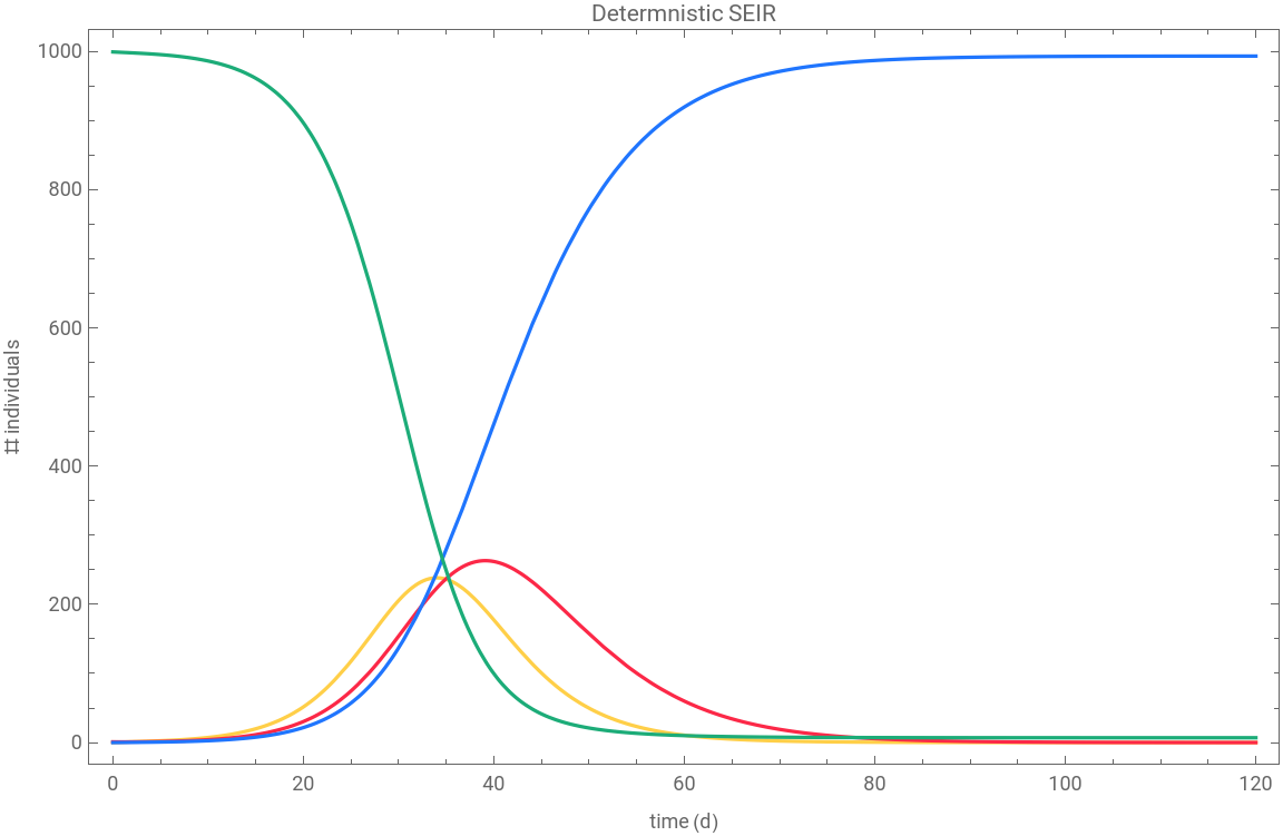


Nothing unusual. There is the outbreak that reaches a maximum around day 40, and nearly everyone in the population gets infected.
Now, let’s see what the stochastic simulation shows. We’ll use the same parameters and the same initial conditions, and run 500 (typically one would use more runs, but we'll keep it on the small side for this essay; we'll also use SeedRandom from time to time) simulations (the code for stochasticSolve is in the initialization section at the end of the notebook).
SeedRandom[1425367]solnsCME=Table[stochasticSolve[modelData["Rates"]/.paramsN,modelData["StoichiometricMatrix"],Through@modelData["Variables"][0]/.Rule@@@inits/.paramsN,modelData["Variables"],{t,0,tmax}],500];//Timing
Out[]=
{35.578,Null}
Here is a plot of the first 20 runs:
epidemicModelPlot[Join@@Take[solnsCME,20],{0,tmax},"modelName"modelName,ImageSizeLarge]
Out[]=
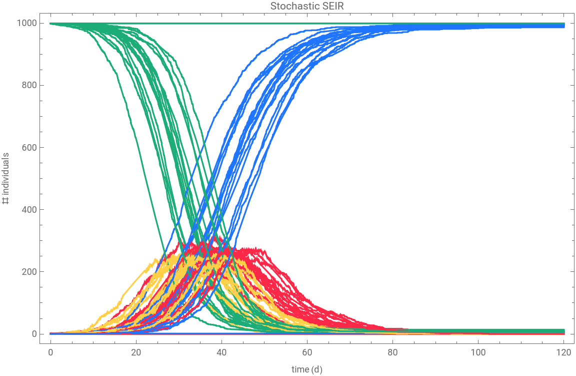
We can see that there is quite a bit of variability in the individual runs, and that there is about a three week variation for the occurrence of the outbreak maximum with possibly a hint of bimodal shape. Moreover, some of the runs did not produce an outbreak. We can examine the average behavior by plotting the median and the middle 95 percentile band:
TabView[{"median with bands"epidemicModelPlot[solnsCME,{0,tmax},"modelName""SIR",ImageSizeLarge],"median"epidemicModelPlot[solnsCME,{0,tmax},"modelName"modelName,ImageSizeLarge,"showBands"False]}]
Out[]=
median with bands
median
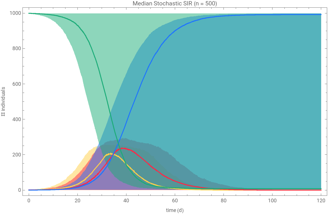
The middle 95 percentile bands show that there is quite a bit of variability in the ensemble of solutions. Looking at the distributions of susceptible and recovered ℛ at we see that there are essentially two kinds of behavior:
t
t
max
Histogram[Quiet[#[tmax]/.solnsCME],{10},ChartStyleepiColor[#],PlotLabel#,PlotRange400,ImageSize4×72]&/@{,ℛ}//Row[#,Spacer[18]]&
Out[]=
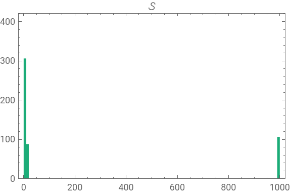

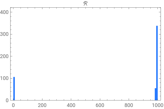
We can partition the ensemble into an “outbreak” and “not an outbreak” subsets:
{outbreak,notOutbreak}=Quiet[SortBy[solnsCME,(ℛ[tmax]/.#)<50&]//SplitBy[#,(ℛ[150]/.#)<50&]&];Length/@%
About a fifth of the time the infection dies out before an outbreak can be established. Now, looking at the average behavior of the outbreak group, while the average behavior is very similar to that for the deterministic solution, the substantial variability remains.
So, why are there two different regimes of behavior? Now would be a good time to examine the Gillespie Algorithm.
Adagio—Details of the Gillespie Algorithm
Adagio—Details of the Gillespie Algorithm
Elements of a stochastic simulation
Elements of a stochastic simulation
The simulation is a Markov chain process, which is a random process that depends only on the current state to determine the next state. The events that occur at step of the chain are the transitions of the SEIR model, in this case. The likelihood of a particular event occurring depends on its propensity, which in turn depends on the current state, that is, the numbers of individuals in each compartment. The time between events depends on the total propensity of the system in the current state. The propensity changes from step to step, and the process ends when the maximum time of the simulation is reached, or when the total propensity is 0.
Computing the propensity
Computing the propensity
To demonstrate the steps, we begin by assuming a current state and time:
The individual propensities define an empirical distribution:
Graphically, we can see how the propensities on the left contribute to the cumulative distribution on the right:
The next state is computed by incrementing the current state with stoichiometry of the selected transition:
The events occur randomly in time, and are therefore a Poisson process. It is the same process followed by radioactive decay, and follows an exponential distribution:
Coding it up
Coding it up
Propensity
Propensity
First, we need to compute the propensity at each step, so let’s make a function that generates the model-specific propensity function. This function will take two arguments: the current state and the current time. We include the time because some models may have time-dependent rates for treatment or mitigation strategies.
For most epidemiology models, the elements of the stoichiometric matrix are 0, 1, or -1, so if one or more of the compartments for a transition are exhausted the resulting propensity for that transition is 0 and that transition cannot be selected—that’s good. However, if the stoichiometry of one of the contributing compartments is 2 or more, then a non-zero propensity will still be computed when there is only 1 individual left in that state, and if that state gets selected, the resulting new state will have a negative entry—that’s not good. So we need to define a model-specific mask function that returns a list of 1’s and 0’s according to whether or not there are sufficient individuals present in the current state to support a transition.
This code generates the propensity function for our SEIR model:
And here is an example of its use:
Simulation loop
Simulation loop
At the end of the simulation, the state vector shows that there are no exposed or infectious individuals, 993 recovered, and 7 susceptible.
Result in same the form as used by NDSolve
Result in same the form as used by NDSolve
Click on the output above to flip between the stochastic and deterministic simulations.
Code optimization
Code optimization
The SEIR model is fairly simple and has an absorbing compartment ℛ (i.e., a sink), so it evaluates fairly quickly, and often terminates before the maximum time threshold is reached. If we use a population 100 times larger it will take much longer to evaluate. Running hundreds or thousands of simulations to study average behavior will take much longer. Finally, a bigger model (e.g., a gene regulatory network or a cell signalling network) will take much longer also. The simulation above took almost 1 second, so just imagine the effect of any one of the above factors on the running time!
There are two bottlenecks in the code:
◼
we can speed up the computation by going to the heart of the matter and skipping the overhead
◼
we can speed up the computation by creating a function with a precomputed body
I won’t go into the details here, but the code in the initialization section at the end of the notebook has been optimized, giving a substantial speed up. It’s still top-level Wolfram Language code, however, and compilation is still and option for further improvement. Here is the usage message for the solver:
Scherzo—Flattening the curve
Scherzo—Flattening the curve
So, back to the SEIR model and the failure to achieve an outbreak in some runs. It all has to do with the probability of infection events happening, and therefore a sufficient number of them relative to the number of recovery events. Recall that the initial state has just one infected individual:
Effectiveness of early international travel restrictions
Effectiveness of early international travel restrictions
Examining how the propensity varies over the time course of the simulation offers some interesting insights. Here is a plot of the individual and total propensities from the first run of the stochastic simulation:
In the early days of the pandemic, international travelers were introducing many more than one infected person into uninfected populations. Here is the effect of starting with 1, 2, 3, 4, or 5 initial infections:
Plotting the fraction of runs that produced an outbreak shows clearly the effect of multiple initiating infectious individuals:
By limiting the number of initial infections, the likelihood of an outbreak is diminished. Below is a comparison of three countries without international travel restrictions to three countries with essentially closed borders. Other factors, such as social distancing, shelter in place, and lock down orders, have also had an effect, and a thorough analysis of all the data is needed before strong conclusions can be made. However, the plots remain suggestive.
Flattening the curve
Flattening the curve
Rondo—Time to achieve eradication
Rondo—Time to achieve eradication
What can we say about the time it takes for the outbreak to die out? The deterministic model gives a very precise answer. Making a semi-log plot makes it easier to seen when the number of exposed and infectious individuals fall below 1.
We need to make another stochastic simulation with the longer simulation time to accurately capture the full time course of each run.
Again, let’s separate into “out break” and “not an outbreak”.
Plotting the average results for the stochastic simulation that had an outbreak shows similar results.
However, showing the individual runs for exposed and infectious shows us something rather different:
Even from just the first 50 runs, we can see that there is quite a bit of variation in the time to become infection-free, and for the infectious compartment ℐ it tends toward longer times.
The key take-aways are 1) the span is quite long, 49 days for the middle 95 percentile, and 2) it has a long tail.
Early data from an epidemic outbreak can be used to fit the parameters for a model using the deterministic simulation. However, the stochastic simulation will give a better estimation of window for when peak is likely to occur, and when the infection-free state might occur. Using parameter confidence intervals from a statistical fit in addition to the inherent variability should give the most realistic estimates.
Summary
Summary
In this short essay I showed how compartmental models can be used for stochastic simulation, in addition to the more traditional deterministic simulation. While the average behavior of many stochastic simulations is essentially the same as for the deterministic simulation, the former reveal that in many cases an epidemic outbreak may fail to materialize.
Finally, I explored the time to achieve an infection-free state following an outbreak, and showed that, in contrast to the deterministic simulation that gives a precise time, the stochastic simulation can give a distribution for that time, allowing one to better predict how long mitigation measures need to be kept in place to minimize morbidity and mortality from COVID-19.
References
References
1
.Daniel T. Gillespie, "Exact Stochastic Simulation of Coupled Chemical Reactions" J. Phys. Chem., 1977, 81, 2340-2361.
2
.Desmond J. Higham, “Modeling and Simulating Chemical Reactions” SIAM Review, 2008, 50, 347-368.
3
.Darren J. Wilkinson, Stochastic Modeling for Systems Biology, Chapman & Hall, Boca Raton, FL 2006.
4
.R. B. Nachbar, J. S. Saltzman, J. A. Stone, and P. Panorchan, “Modeling HCV Clinical Trial Outcomes With Hybrid Deterministic-Stochastic Methods” presented at the SIAM Life Science 2010 Conference, Pittsburgh, PA, 12-15 July 2010. http://www.siam.org/meetings/ls10/LS10_abstracts.pdf
5
.Robert Nachbar and Jeffrey Saltzman, “Hybrid Deterministic-Stochastic Modeling—Using Differential Equations and the Chemical Master Equation” presented at the Wolfram Technology Conference 2012, Wolfram Research Inc., Champaign, IL, 17-19 October 2012. https://library.wolfram.com/infocenter/Conferences/8725/
CITE THIS NOTEBOOK
CITE THIS NOTEBOOK
Stochastic Epidemiology Models with Applications to the COVID-19
by Robert Nachbar
Wolfram Community, STAFF PICKS, 2020
https://community.wolfram.com/groups/-/m/t/1980051
by Robert Nachbar
Wolfram Community, STAFF PICKS, 2020
https://community.wolfram.com/groups/-/m/t/1980051