Bernd Mulansky, January 2024
Some peculiarities of GeneralMiniMaxApproximation
Some peculiarities of GeneralMiniMaxApproximation
In[]:=
$Version
Out[]=
14.0.0 for Mac OS X ARM (64-bit) (December 13, 2023)
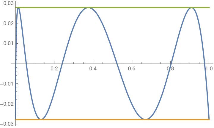
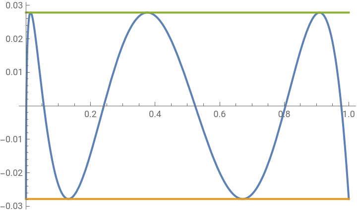
Throughout this notebook we use the function from the repository, ensured by a fresh kernel. At first we compute the best minimax approximation to the square root function on [0,1] by a polynomial of degree 5. Since we want to minimize the absolute error we have to use GeneralMiniMaxApproximation. So the square root function can be defined explicitly or implicitly. Both variants work quite well. They give identical solutions showing the characterizing Chebyshev alternant of the error.
In[]:=
gma=ResourceFunction["GeneralMiniMaxApproximation"];sqrexRF=gma[{t,Sqrt[t],1},{t,{0,1},5,0},t]sqrimRF=gma[{t^2,t,1},{t,{0,1},5,0},t]
Out[]=
{{0.,0.0142025,0.131525,0.375967,0.671397,0.909262,1.},{0.0278451+4.75365t-20.6463+47.7753-49.5921+18.7094,-0.0278451}}
2
t
3
t
4
t
5
t
Out[]=
{{0.,0.119174,0.362664,0.613161,0.819388,0.953552,1.},{0.0278451+4.75365t-20.6463+47.7753-49.5921+18.7094,-0.0278451}}
2
t
3
t
4
t
5
t
In[]:=
Plot[{Sqrt[t]-sqrexRF[[2,1]],sqrexRF[[2,2]],-sqrexRF[[2,2]]},{t,0,1}]Plot[{Sqrt[t]-sqrimRF[[2,1]],sqrimRF[[2,2]],-sqrimRF[[2,2]]},{t,0,1}]
Out[]=
Out[]=
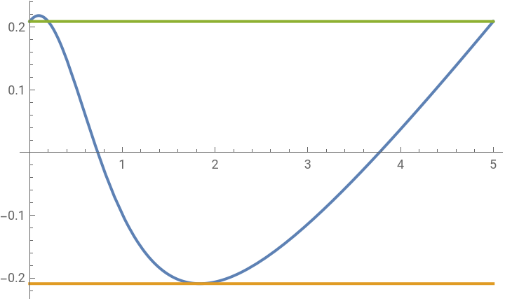
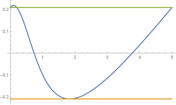
Now we compute the minimax approximation to the celebrated Runge function on [0,5] by a linear polynomial. The result is wrong, as the error function reveals.
In[]:=
runge[t_]=1/(1+t^2);ruRF=gma[{t,runge[t],1},{t,{0,5},1,0},t]Plot[{runge[t]-ruRF[[2,1]],-ruRF[[2,2]],ruRF[[2,2]]},{t,0,5}]
Out[]=
{{0.,1.83552,5.},{0.790931-0.192308t,0.209069}}
Out[]=
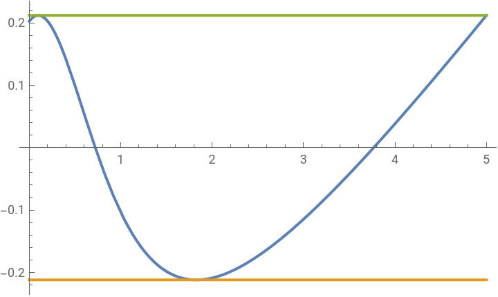
The correct polynomial is (up to the shown precision)
In[]:=
ruc[t_]=0.7974355-0.1942119t;
with the error
In[]:=
ec=MaxValue[{Abs[runge[t]-ruc[t]],0≤t≤5},t]Plot[{runge[t]-ruc[t],-ec,ec},{t,0,5}]
Out[]=
0.212086
Out[]=
Minimax approximation by polynomials of degree 2 and 3 fails.
In[]:=
gma[{t,runge[t],1},{t,{0,5},#1,0},t]&/@{2,3}
Out[]=
{{{0.,1.26814,3.63466,5.},1.07648-0.553342t+0.0711682,{-0.0764835,-0.105811,0.0649082,-0.05052}},{{0.,0.465678,2.52584,4.24416,5.},1.11311-0.818665t+0.217219-0.0194054,{-0.113111,0.0447673,0.0170886,-0.0151807,0.0138713}}}
2
t
2
t
3
t
In[]:=
gma[{t,runge[t],1},{t,{0,5},#1,0},t,Brake->{12,10}]&/@{2,3}
Out[]=
{{{0.,1.26814,3.63466,5.},1.07648-0.553342t+0.0711682,{-0.0764835,-0.105811,0.0649082,-0.05052}},{{0.,0.465678,2.52584,4.24416,5.},1.11311-0.818665t+0.217219-0.0194054,{-0.113111,0.0447673,0.0170886,-0.0151807,0.0138713}}}
2
t
2
t
3
t
Surprisingly, degrees 4 and 5 are okay.
In[]:=
ru45=gma[{t,runge[t],1},{t,{0,5},#1,0},t]&/@{4,5}
Out[]=
{{{0.,0.317373,1.16578,2.66237,4.29528,5.},{1.03755-0.521307t-0.0268552+0.0506225-0.00653845,-0.0375467}},{{0.,0.28771,0.985806,2.09825,3.45539,4.57095,5.},{1.02155-0.318552t-0.417692+0.30002-0.0691805+0.00537884,-0.0215477}}}
2
t
3
t
4
t
2
t
3
t
4
t
5
t
In[]:=
Plot[{runge[t]-ru45[[2,2,1]],ru45[[2,2,2]],-ru45[[2,2,2]]},{t,0,5}]
Out[]=
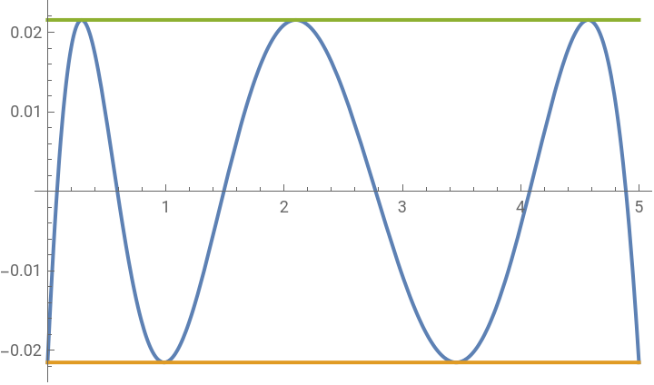
Or not so surprising? There seem to be problems if the interval boundaries do not belong to the extrema of the error of the best minimax approximation. Let’s try to find out. As we see, the first and last abscissa of the alternant are pinned at the interval boundaries.
In[]:=
ru1=gma[{t,runge[t],1},{t,{0,5},1,0},t,Bias->-0.2,PrintFlag->True,PlotFlag->True]Plot[{runge[t]-ru1[[2,1]],-ru1[[2,2]],ru1[[2,2]]},{t,0,5}]
{0.177172}
{0.0262981}
{0.000812651}
{7.51349×}
-7
10
{6.41556×}
-13
10
{{0.,0.0859678},{1.74629,-0.295168},{5.,0.189321}}
{0.0113536}
{{0.,0.11517},{1.76635,-0.27461},{5.,0.193915}}
{0.013291}
{{0.,0.148609},{1.79014,-0.251175},{5.,0.199231}}
{0.0135807}
{{0.,0.182134},{1.81479,-0.22779},{5.,0.204633}}
{0.00934309}
{{0.,0.20456},{1.8319,-0.212202},{5.,0.208309}}
{0.00196815}
{{0.,0.209068},{1.83552,-0.209069},{5.,0.209068}}
{4.67632×}
-6
10
Out[]=
{{0.,1.83552,5.},{0.790931-0.192308t,0.209069}}
Out[]=
See also runge_minimax _Package _ 2024. nb