Extractive distillation is one of several methods that can be used to separate an azeotropic mixture Ref. 1-2. In extractive distillation a third component, called an entrainer, is added to the mixture to break the azeotrope.
Following Ref. 3, the feed to the extractive distillation column is an equimolar mixture of isopropyl alcohol (IPA) and water using dimethyl sulfoxide (DMSO) as an entrainer. The column has 41 equilibrium stages, a partial reboiler, and a total condenser. The feed locations for the entrainer and-water mixture are stages 7 and 35, respectively. (Stages are counted from the top of the column.) The DMSO feed flow is 1708.33 kmol/hr, and the azeotropic mixture (IPA and water) feed flow rate is 1666.67 kmol/hr. For a well-posed problem, we set the distillate flow rate equal to 832.50 kmol/hr and set the reflux stream flow rate to 527.81 kmol/hr.
Following Ref. 3, the feed to the extractive distillation column is an equimolar mixture of isopropyl alcohol (IPA) and water using dimethyl sulfoxide (DMSO) as an entrainer. The column has 41 equilibrium stages, a partial reboiler, and a total condenser. The feed locations for the entrainer and
IPA
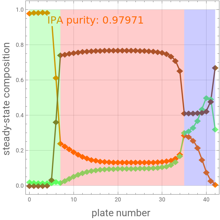
We compute the composition and temperature profiles inside the extractive distillation column. In the composition profile plots, the orange, brown, and green curves correspond to the compositions of IPA, DMSO, and water, respectively. You can easily see that the highest concentration of IPA (almost 100 mole %) is obtained for low entrainer feed temperatures 345.15 Kelvin. If the entrainer temperature is increased, the separation becomes less efficient, and the purity of IPA leaving the top of the column decreases.
We check our results against those given by Aspen HYSYS.
We check our results against those given by Aspen HYSYS.
The various functions of the extractive column can be described as follows: in the rectifying section of the column (above the entrainer feed location) the IPA mixture is purified (little if any water or DMSO is present), while in the stripping section of the column (below the azeotropic mixture feed location) IPA is stripped from the mixture. In the section of the column between the two feeds (also called the extractive section), a high DMSO composition is present. These features are evident on the composition plots.
The bottom product of the extractive distillation column is DMSO and water. DMSO is separated from water in a solvent recovery column (not shown), cooled, and then recycled back to the extractive distillation column.
The bottom product of the extractive distillation column is DMSO and water. DMSO is separated from water in a solvent recovery column (not shown), cooled, and then recycled back to the extractive distillation column.
Expressions for pure component vapor and liquid enthalpies were adapted from Aspen HYSYS. The mixture is assumed to obey the modified Raoult's law and activity coefficients are predicted using the Wilson model [4].
Total pressure
In[]:=
P=101.325;
Constants for the Modified Antoine Equation (obtained from HYSYS)
In[]:=
A1=83.6370;B1=-8249.010;C1=0.;D1=-9.545180;E1=2.002720/10^6;F1=2.;A2=65.9278;B2=-7227.53;C2=0.;D2=-7.17695;E2=4.0313/10^6;F2=2.;A3=49.3650;B3=-7620.60;C3=0.;D3=-4.62790;E3=4.38180/10^7;F3=2.;PSat[1][i_]:=Exp[A1+B1/(C1+T)+D1*Log[T]+E1*T^F1]/.TT[i];PSat[2][i_]:=Exp[A2+B2/(C2+T)+D2*Log[T]+E2*T^F2]/.TT[i];PSat[3][i_]:=Exp[A3+B3/(C3+T)+D3*Log[T]+E3*T^F3]/.TT[i];
Expressions for the pure components liquid-phase and vapor-phase enthalpies (obtained from Aspen-HYSYS)
In[]:=
a1=0.;b1=342.7726;c1=-1.431749;d1=3.520110/10^3;e1=-2.5597070/10^6;h1=a1+b1*T+c1*T^2+d1*T^3+e1*T^4/.T273.15;hl1=a1+b1*T+c1*T^2+d1*T^3+e1*T^4-h1;a2=0.;b2=76.28204;c2=2.565142/10^2;d2=-1.127938/10^4;e2=1.325963/10^7;h2=a2+b2*T+c2*T^2+d2*T^3+e2*T^4/.T273.15;hl2=a2+b2*T+c2*T^2+d2*T^3+e2*T^4-h2;a3=0.;b3=240.3001;c3=-0.2975006;d3=3.3766780/10^4;e3=-8.24960/10^13;h3=a3+b3*T+c3*T^2+d3*T^3+e3*T^4/.T273.15;hl3=a3+b3*T+c3*T^2+d3*T^3+e3*T^4-h3;a1v=52000.86;b1v=462.877800;c1v=-2.41189;d1v=5.8568160/10^3;e1v=-4.8396590/10^6;Hv1=a1v+b1v*T+c1v*T^2+d1v*T^3+e1v*T^4-h1;a2v=47304.17;b2v=107.5791;c2v=-0.2202581;d2v=3.661611/10^4;e2v=-3.228085/10^7;Hv2=a2v+b2v*T+c2v*T^2+d2v*T^3+e2v*T^4-h2;a3v=65684.10;b3v=211.21310;c3v=-0.3536537;d3v=4.2391060/10^4;e3v=-1.0486910/10^7;Hv3=a3v+b3v*T+c3v*T^2+d3v*T^3+e3v*T^4-h3;
Mixture liquid-phase and vapor-phase enthalpies
In[]:=
H[i_]:=y[1][i]*Hv1+y[2][i]*Hv2+y[3][i]*Hv3/.TT[i];h[i_]:=x[1][i]*hl1+x[2][i]*hl2+x[3][i]*hl3/.TT[i];
Universal gas constant in kcal/K*kmol
In[]:=
R=1.987;
Activity coefficients using Wilson Model
In[]:=
a[1,1]=0;a[1,2]=789.707153320313;a[1,3]=-559.149414062500;a[2,1]=1010.50030517578;a[2,2]=0;a[2,3]=47.1153717041016;a[3,1]=148.309570312500;a[3,2]=-929.458374023438;a[3,3]=0;Vw[1]=7.75554297348814;Vw[2]=1.78833825504182;Vw[3]=7.12092691060110;Gam[i_,k_]:=Exp[1-Log[Sum[x[j][k]*Aw[i,j,k],{j,1,3}]]-Sum[(x[p][k]*Aw[p,i,k])/Sum[x[j][k]*Aw[p,j,k],{j,1,3}],{p,1,3}]];Aw[i_,j_,k_]:=(Vw[j]/Vw[i])*Exp[-a[i,j]/(R*T[k])];
Upper-feed and lower-feed temperatures
In[]:=
TFU=345.15;
In[]:=
TFL=82.53+273.15;
Upper-feed and lower-feed stream enthalpies
In[]:=
hFU=zU[1]*hl1+zU[2]*hl2+zU[3]*hl3/.TTFU;hFL=zL[1]*hl1+zL[2]*hl2+zL[3]*hl3/.TTFL;
summation rules
In[]:=
y[3][i_]:=1-y[1][i]-y[2][i];x[3][i_]:=1-x[1][i]-x[2][i];
distillate stream enthalpy
In[]:=
h[0]=y[1][1]*hl1+y[2][1]*hl2+y[3][1]*hl3/.TT[0];
Upper-feed and lower-feed flow rates
In[]:=
FU=1708;
In[]:=
FL=1667;
Upper-feed and lower-feed composition
In[]:=
zU[1]=0;zU[2]=0;zU[3]=1;
In[]:=
zL[1]=0.5;zL[2]=0.5;zL[3]=0;
MESH equations
In[]:=
eq1=Di+L[0]V[1];eq2=Di*h[0]+L[0]*h[0]V[1]*H[1]+Qc;eq3[i_]:=V[i]+L[i]V[i+1]+L[i-1];eq4[i_]:=Table[V[i]*y[j][i]+L[i]*x[j][i]V[i+1]*y[j][i+1]+L[i-1]*x[j][i-1],{j,1,2}];eq5[i_]:=Table[y[j][i]*Px[j][i]*PSat[j][i]*Gam[j,i],{j,1,2}];eq6[i_]:=V[i]*H[i]+L[i]*h[i]V[i+1]*H[i+1]+L[i-1]*h[i-1];eq7=V[7]+L[7]-FUV[8]+L[6];eq8=Table[V[7]*y[i][7]+L[7]*x[i][7]-FU*zU[i]V[8]*y[i][8]+L[6]*x[i][6],{i,1,2}];eq9=Table[y[i][7]*Px[i][7]*PSat[i][7]*Gam[i,7],{i,1,2}];eq10=V[7]*H[7]+L[7]*h[7]-FU*hFUV[8]*H[8]+L[6]*h[6];eq11=V[35]+L[35]-FLV[36]+L[34];eq12=Table[V[35]*y[i][35]+L[35]*x[i][35]-FL*zL[i]V[36]*y[i][36]+L[34]*x[i][34],{i,1,2}];eq13=Table[y[i][35]*Px[i][35]*PSat[i][35]*Gam[i,35],{i,1,2}];eq14=V[35]*H[35]+L[35]*h[35]-FL*hFLV[36]*H[36]+L[34]*h[34];eq15=V[42]+BL[41];eq16=Table[V[42]*y[i][42]+B*x[i][42]L[41]*x[i][41],{i,1,2}];eq17=Table[y[i][42]*Px[i][42]*PSat[i][42]*Gam[i,42],{i,1,2}];eq18=V[42]*H[42]+B*h[42]L[41]*h[41]+Qr;eq19=L[0]527.8;(*giveninproblemstatement*)eq20=Di832.50;(*giveninproblemstatement*)eq21=Table[Sum[x[i][j]*PSat[i][j]*Gam[i,j],{i,1,3}]P,{j,0,42}];eq22=Table[x[i][0]y[i][1],{i,1,2}];
Solution of MESH Equations (301 nonlinear algebraic equations) using FindRoot
In[]:=
sys=Flatten[{eq1,eq2,Table[{eq3[i],eq4[i],eq5[i],eq6[i]},{i,1,6}],Table[{eq3[i],eq4[i],eq5[i],eq6[i]},{i,8,34}],Table[{eq3[i],eq4[i],eq5[i],eq6[i]},{i,36,41}],eq15,eq16,eq17,eq18,eq19,eq20,eq21,eq22,eq7,eq8,eq9,eq10,eq11,eq12,eq13,eq14}];
In[]:=
Length[sys]
Out[]=
301
In[]:=
Column composition profile (liquid-phase) (our results versus Aspen-HYSYS results). Excellent agreement between both sets of data is found.
In[]:=
plcp=ListPlot[{Table[{i,x[1][i]}/.sol1,{i,0,42}],Table[{i,x[2][i]}/.sol1,{i,0,42}],Table[{i,x[3][i]}/.sol1,{i,0,42}]},PlotMarkers{"◆",16},AxesOrigin{0,0},JoinedTrue,FrameLabel{Style["plate number ",16],Style["steady-state composition ",16]},FrameTrue,GridLinesAutomatic,PlotStyle{{Thick,Orange},{Thick,RGBColor[0.47,1,0.47]},{Thick,Brown}},ImageSize{350,350},AspectRatio1,PlotRange{-0.05,1.05},Epilog{Style[Text[Row[{"IPA purity: ",NumberForm[x[1][0]/.sol1,{6,5}]}],{15,0.94}],BackgroundWhite,Orange,16],Opacity[0.2],Green,Rectangle[{0,0},{7,1}],Red,Rectangle[{7,0},{35,1}],Blue,Rectangle[{35,0},{42,1}]}]
Out[]=
In[]:=
plcp2=ListPlot[{Table[{i,x[1][i]}/.sol1,{i,0,42}],Table[{i,x[2][i]}/.sol1,{i,0,42}],Table[{i,x[3][i]}/.sol1,{i,0,42}]},JoinedTrue,FrameLabel{Style["plate number ",16],Style["steady-state composition ",16]},FrameTrue,GridLinesAutomatic,PlotStyle{{Thickness[0.0075],Black,Dashed},{Thickness[0.0075],Black,Dashed},{Thickness[0.0075],Black,Dashed}},ImageSize{350,350},AspectRatio1,PlotRange{{0,42},{0.0,1.0}}]
Column temperature profile (our results versus Aspen-HYSYS results). Excellent agreement between both sets of data is found.
Column composition profile (vapor-phase) (our results versus Aspen-HYSYS results). Excellent agreement between both sets of data is found.
References
References
◼
[1] M. F. Doherty and M. F. Malone, Conceptual Design of Distillation Systems, Boston: McGraw-Hill, 2001.
◼
[2] E. J. Henley and J. D. Seader, Equilibrium-Stage Separation Operations in Chemical Engineering, New York: Wiley, 1981.
◼
[3] W. L. Luyben and I.-L. Chien, Design and Control of Distillation Systems for Separating Azeotropes, Hoboken, NJ: Wiley, 2010.
◼
[4] G. M. Wilson, "Vapor-Liquid Equilibrium XI: A New Expression for the Excess Free Energy of Mixing," Journal of the American Chemical Society, 86(2), 1964 pp. 127–130.
CITE THIS NOTEBOOK
CITE THIS NOTEBOOK
Extractive Distillation of Azeotorpic Mixture using Wolfram Language versus its Counterpart by HYSYS
by Housam Binous and Ahmed Bellagi
Wolfram Community, STAFF PICKS, February 8, 2024
https://community.wolfram.com/groups/-/m/t/3114693
by Housam Binous and Ahmed Bellagi
Wolfram Community, STAFF PICKS, February 8, 2024
https://community.wolfram.com/groups/-/m/t/3114693