1 Introduction
1 Introduction
The spring-mass-damper system is one of the fundamental models in the study of mechanical vibrations, as it describes the motion of a mass attached to a spring and subjected to a damping force that represents energy dissipation due to effects such as friction or resistance. The motion is assumed to occur in a single direction, making the system one-dimensional. According to Newton’s second law, the equation of motion governing this system is given by: , where all derivatives are taken with respect to time . Here, represents the displacement of the mass as a function of time, denotes the mass of the system, is the damping coefficient, and is the spring stiffness constant. The term represents the inertial force, corresponds to the damping force opposing the motion, and ) represents the restoring force exerted by the spring.
my''(t)+cy'(t)+ky(t)=0
t
y(t)
m
c
k
my''(t)
cy'(t)
ky(t
Determine the second-order homogeneous differential equation governing the free motion of the damped spring–mass–damper system:
In[]:=
eqnGeneral=my''[t]+cy'[t]+ky[t]0;
Based on the value of the damping coefficient , the system’s motion is broadly classified into two primary regimes. In the absence of damping , the system is undamped and exhibits purely oscillatory motion with no energy dissipation. In contrast, when damping is present , the system’s dynamic response is governed by the discriminant . Accordingly, the damped motion is categorized into three distinct regimes: overdamped, critically damped , and underdamped , each exhibiting qualitatively different dynamic behavior. The following tree diagram illustrates this classification along with the corresponding motion types. This framework is derived from the discriminant of the characteristic equation, which fundamentally determines the nature of the system’s response.
c
(c=0)
(c≠0)
Δ=−4mk
2
c
(Δ>0)
(Δ=0)
(Δ<0)
In[]:=
Graph,
Out[]=
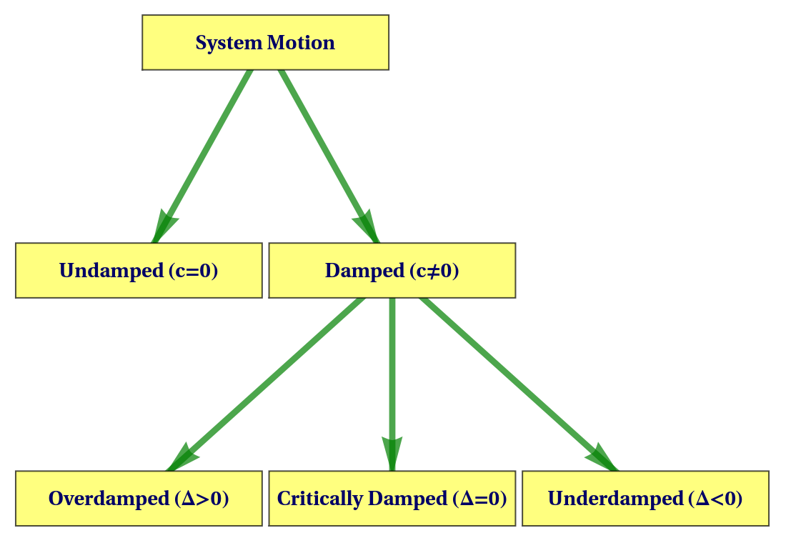
The general formulation of the spring–mass–damper system has been presented along with its classification into undamped and damped motions based on the system parameters. Accordingly, each case will be examined in detail, where the displacement, velocity, and acceleration will be derived for every type of motion. Furthermore, the energy behavior will be analyzed in terms of kinetic energy, potential energy, and energy dissipation, supported by graphical representations and illustrative examples for each case.
2 Undamped Motion
2 Undamped Motion
In this section, the undamped mass-spring system is analyzed, where the damping coefficient , representing an ideal frictionless scenario. The displacement is derived, followed by the computation of kinetic and potential energies. It is then shown that the total mechanical energy remains constant over time. To validate these theoretical results, a numerical example with physically meaningful parameters is presented, illustrating the periodic motion and confirming energy conservation through analytical expressions and graphical visualization.
c=0
y(t)
Set the damping coefficient to zero to represent the undamped harmonic motion equation:
c
In[]:=
eqnUndamped=eqnGeneral/.c0
Out[]=
ky[t]+m[t]0
′′
y
This second-order linear differential equation corresponds to simple harmonic motion, where the restoring force is proportional to the displacement and acts in the opposite direction.
Solve the undamped motion equation, replacing constants , with and , and with ω:
1
2
A
B
k
m
In[]:=
yUndamped[t_]=DSolveValue[eqnUndamped,y[t],t]/.A,B,ω
1
2
k
m
Out[]=
ACos[tω]+BSin[tω]
In the undamped case, represents the initial displacement, while is related to the initial velocity and is given by .
A
B
B=v(0)/ω
Derive the velocity function by differentiating the undamped displacement with respect to time:
v(t)
y(t)
In[]:=
vUndamped[t_]:=yUndamped'[t];vUndamped[t]
Out[]=
BωCos[tω]-AωSin[tω]
Derive the acceleration function by differentiating the undamped displacement twice with respect to time:
a(t)
y(t)
In[]:=
aUndamped[t_]:=yUndamped''[t];aUndamped[t]
Out[]=
-ACos[tω]-BSin[tω]
2
ω
2
ω
The acceleration is proportional to the negative displacement, confirming that the motion is oscillatory and directed toward the equilibrium position.
Determine the kinetic energy function for the undamped system:
K(t)
In[]:=
kEUndamped[t_]:=m;kEUndamped[t]
1
2
2
vUndamped[t]
Out[]=
1
2
2
(BωCos[tω]-AωSin[tω])
Determine the potential energy of the undamped system:
In[]:=
pEUndamped[t_]:=Simplifyk;pEUndamped[t]
1
2
2
yUndamped[t]
Out[]=
1
2
2
(ACos[tω]+BSin[tω])
Define the total mechanical energy function :
E(t)
In[]:=
tEUndamped[t_]:=kEUndamped[t]+pEUndamped[t];tEUndamped[t]
Out[]=
1
2
2
(ACos[tω]+BSin[tω])
1
2
2
(BωCos[tω]-AωSin[tω])
To verify that the total energy of the undamped system is constant and independent of time, two methods are employed. First, trigonometric simplification is performed using TrigReduce, which reduces the energy expression to a time-independent form. Second, the total energy is differentiated with respect to time to check its independence from time. These results confirm that the total energy remains constant over time.
In[]:=
TrigReducetEUndamped[t]/.{ω->
k/m
}Out[]=
1
2
2
A
2
B
Simplify the derivative of the undamped total energy after substituting :
ω=
k/m
In[]:=
SimplifytEUndamped'[t]/.ω
k
m
Out[]=
0
The results confirm that the total energy of the undamped system is independent of time and remains constant.
To illustrate the theoretical results, we consider a practical example of an undamped mass–spring system. An iron ball weighing extends the spring by from its natural length.. The motion of the system is studied when the ball is released from rest from a position below the equilibrium position, with zero initial velocity.
9.8N
1.09m
1.2m
Assign the weight, spring extension, and gravitational acceleration values:
In[]:=
w=9.8;ΔS=1.09;g=9.8;
From the given example, the mass and spring constant are obtained using and , respectively.
m=w/g
k=w/ΔS
Assign , , and ω from weight and spring extension, where :
m
k
ω=
k/m
In[]:=
paramsUndamped=mwg,kwΔS,ω
w/ΔS
w/g
Out[]=
{m1.,k8.99083,ω2.99847}
Determine the period :
T
In[]:=
T=/.ω/.{k->w/ΔS,mw/g}
2π
ω
k
m
Out[]=
2.09546
Determine the frequency :
f
In[]:=
f=/.ω/.{k->w/ΔS,mw/g}
ω
2π
k
m
Out[]=
0.477221
Apply the initial conditions (position and rest) to find the specific values for constants and Β:
Α
In[]:=
constantsSol=Solve[{yUndamped[0]1.2,vUndamped[0]0},{A,B}][[1]]//N
Out[]=
{A1.2,B0.}
Compute the undamped displacement by substituting parameters and evaluating numerically:
In[]:=
yUndampedMotion[t_]:=yUndamped[t]/.A1.2,B0,ω/.{mw/g,kw/ΔS};yUndampedMotion[t]
k
m
Out[]=
1.2Cos[2.99847t]
Determine the undamped velocity by substituting the constants and system parameters and expanding the expression:
In[]:=
vUndampedMotion[t_]:=Chop@ExpandvUndamped[t]/.A1.2,B0,ω/.{mw/g,kw/ΔS};vUndampedMotion[t]
k
m
Out[]=
-3.59816Sin[2.99847t]
Determine the undamped acceleration by substituting the constants and system parameters, then expand and simplify the expression:
In[]:=
aUndampedMotion[t_]:=SimplifyExpandaUndamped[t]/.A1.2,B0,ω/.{mw/g,kw/ΔS};aUndampedMotion[t]
k
m
Out[]=
-10.789Cos[2.99847t]
Determine the kinetic energy of the undamped system by substituting the constants and system parameters and expanding the expression:
In[]:=
kEUndampedMotion[t_]:=Chop@ExpandkEUndamped[t]/.A1.2,B0,ω/.{mw/g,kw/ΔS};kEUndampedMotion[t]
k
m
Out[]=
6.47339
2
Sin[2.99847t]
Determine the potential energy of the undamped system by substituting the constants and system parameters and expanding the expression:
In[]:=
pEUndampedMotion[t_]:=ExpandpEUndamped[t]/.A1.2,B0,ω/.{mw/g,kw/ΔS};pEUndampedMotion[t]
k
m
Out[]=
6.47339
2
Cos[2.99847t]
Determine the total mechanical energy of the undamped system by substituting the constants and system parameters and simplifying the expression:
In[]:=
tEUndampedMotion[t_]:=SimplifytEUndamped[t]/.A1.2,B0,ω/.{mw/g,kw/ΔS};tEUndampedMotion[t]
k
m
Out[]=
6.47339
This constant value represents the total mechanical energy of the system, which remains unchanged throughout the motion, confirming the conservation of energy numerically.
Determine custom time-axis tick marks for one oscillation period:
Visualize the system behavior by plotting displacement, velocity and acceleration:
The displacement, velocity, and acceleration of the undamped system are displayed together, providing a comprehensive view of the motion. Initially, the displacement exhibits a smooth sinusoidal oscillation with a constant amplitude, reflecting perfectly periodic behavior. Meanwhile, the velocity oscillates as well, but it is phase-shifted relative to displacement, reaching its maximum as the mass passes through the equilibrium position. Furthermore, the acceleration remains proportional to and opposite in direction to the displacement, confirming the restoring force exerted by the spring. Overall, these three quantities collectively illustrate the characteristics of simple harmonic motion, highlighting the continuous interplay between position, speed, and acceleration in an undamped system.
Visualize the system behavior by plotting energy:
The energy plot shows the kinetic energy (KE) and potential energy (PE) oscillating periodically, demonstrating the continuous exchange between motion and position. While each form of energy varies with time, the total mechanical energy (TE) remains constant throughout the motion. This confirms that, in an ideal undamped system, energy is perfectly conserved and no dissipation occurs. The plot thus provides a clear visualization of energy conservation in harmonic motion. Overall, these plots provide clear analytical and visual confirmation that the undamped system undergoes ideal harmonic motion with constant total energy and sustained oscillations.
In the undamped case, no energy is lost and the system’s total mechanical energy remains constant during motion. This idealized model provides a fundamental reference for studying more realistic damped systems. On this basis, damped motion is examined with emphasis on how damping affects both the dynamics of the system and its energy behavior. In these cases, resistive forces—known as damping forces—are introduced, since energy is gradually dissipated due to friction or air resistance, resulting in a progressive reduction of the oscillation amplitude over time.
3 Overdamped Motion
3 Overdamped Motion
Now, we examine how the total energy change compares with the damping power. Let’s see if the rate of change of total energy equals the instantaneous power lost due to damping.
Determine the specific overdamped displacement by substituting the given parameter values and constants into the general overdamped solution:
Determine the system velocity by substituting the given parameter values and constants into the general overdamped velocity function:
Determine the system acceleration by substituting the given parameter values and constants into the general overdamped acceleration function:
Calculate the kinetic energy by substituting the given parameter values and constants into the general overdamped energy expression:
Evaluate the potential energy by substituting the given parameter values and constants into the general overdamped energy expression:
Determine the total mechanical energy by substituting the given parameter values and constants into the general overdamped energy expression:
Determine the instantaneous power dissipated by substituting the given parameter values and constants into the general overdamped power expression:
Calculate the rate of energy decay by substituting the given parameter values and constants into the general overdamped energy decay expression:
Verify energy consistency by subtracting the instantaneous power from the overdamped energy decay:
Visualize the system behavior by plotting displacement, velocity and acceleration:
Visualize the system behavior by plotting energy:
Although the analytical results confirm the agreement between the damping power and the rate of energy decay, the plots are presented to provide a clear visual verification of this relationship. This graphical representation supports the theoretical conclusion that energy dissipation is governed by the damping force, ensuring consistency between the mathematical model and its physical interpretation in the overdamped regime.
Visualize the system behavior by plotting power over time:
After analyzing the overdamped case, it is observed that the system approaches equilibrium without oscillation, thereby setting the stage for examining the critically damped case, which represents the precise threshold between oscillatory and non-oscillatory motion.
4 Critically Damped Motion
4 Critically Damped Motion
The solution contains a linear term in time multiplied by an exponential decay, which is characteristic of the critically damped case.
The total mechanical energy is not conserved due to the presence of the damping force, which continuously dissipates energy.
Verify that the difference between the energy decay EDecayCriticallyDamped[t] and the damping power powerCriticallyDamped[t] simplifies to zero:
Solve for the integration constants using the initial conditions :
Verify that the rate of change of total energy is equal to the negative damping power:
Visualize the system behavior by plotting displacement, velocity and acceleration:
The plots indicate that the displacement decays smoothly and monotonically toward equilibrium without oscillations or overshoot, consistent with critically damped behavior. The velocity starts from zero, then changes sign once due to the non-oscillatory transient motion, before decaying to zero as equilibrium is approached. The acceleration shows a short transient phase followed by rapid decay. Overall, the results confirm efficient energy dissipation and a non-oscillatory return to equilibrium.
Visualize the system behavior by plotting energy:
From the energy plots, both kinetic and potential energies decay smoothly over time, reflecting the rapid dissipation of mechanical energy under critical damping. There is no oscillatory exchange between kinetic and potential energy; instead, both components decrease monotonically due to the presence of strong damping. Initially, energy is distributed between kinetic and potential forms, but this exchange does not persist, and no sustained oscillations occur. As a result, the total mechanical energy decreases steadily and continuously, confirming an efficient, non-oscillatory return of the system to equilibrium.
Although the analytical results confirm the exact agreement between the damping power and the rate of energy decay, the plots are presented to provide a clear visual verification of this relationship. This graphical representation further supports the theoretical conclusion that energy dissipation is directly governed by the damping force, ensuring consistency between the mathematical model and its physical interpretation.
Visualize the system behavior by plotting power over time:
From the plots, both curves decrease smoothly and exhibit close agreement, confirming that energy loss is governed by the damping force. This demonstrates efficient, non-oscillatory energy dissipation and a smooth convergence toward equilibrium, in agreement with the theoretical model.
Following the analysis of the critically damped system, which returns to equilibrium without oscillations, we proceed to examine the underdamped case, characterized by oscillatory motion with gradually diminishing amplitude.
5 Underdamped Motion
5 Underdamped Motion
To obtain a more physically interpretable form of the solution and to facilitate graphical representation, the complex exponential form is rewritten. This corresponds to complex conjugate roots of the characteristic equation, leading to oscillatory motion and yielding a damped sinusoidal function consistent with the expected behavior of the system.
Calculate and simplify the potential energy pEUnderdamped[t] using the displacement yUnderdamped[t]:
Sum the kinetic and potential energies to calculate the total mechanical energy tEUnderdamed for the Underdamped case:
The total mechanical energy exhibits an overall exponential decay due to damping, while small oscillatory variations arise from the continuous exchange between kinetic and potential energy.
Compute the damping power powerUnderDamped[t] using the velocity vUnderDamped[t]:
The negative sign indicates continuous energy dissipation due to the damping force, where mechanical energy is gradually converted into thermal energy. This confirms that damping does not violate the principle of energy conservation; instead, it represents a redistribution of energy from the mechanical system to the surrounding medium.
Differentiate the total energy tEUnderDamped[t] to obtain the energy decay rate EDecayUnderDamped[t]:
confirming that the damping force fully accounts for energy dissipation in the system.
Compute the total energy of the underdamped system as the sum of kinetic and potential energy:
Verify the equivalence between energy decay rate and damping power by simplifying their difference to zero:
Visualize the system behavior by plotting displacement, velocity and acceleration:
These plots illustrate the kinematic behavior of the underdamped mass–spring–damper system. The displacement exhibits oscillatory motion with an exponentially decaying amplitude due to the presence of damping. The velocity follows a similar oscillatory pattern with a phase shift, reaching its maximum as the system passes through the equilibrium position, reflecting the continuous exchange between kinetic and potential energy. The acceleration also oscillates with decreasing amplitude under the combined influence of the restoring and damping forces. Overall, the system undergoes pseudo-periodic motion with gradually diminishing amplitude, which motivates the subsequent analysis of energy.
Visualize the system behavior by plotting energy:
This plot presents the time evolution of kinetic, potential, and total mechanical energies. The kinetic and potential energies oscillate and continuously exchange roles, with potential energy maximized at peak displacement and kinetic energy dominant near the equilibrium position. In contrast, the total mechanical energy decays exponentially over time due to damping, indicating continuous energy loss from the system. This observed decay motivates a closer examination of the rate of energy dissipation and its physical origin.
Although the analytical results confirm the exact equivalence between damping power and energy decay rate, the plot is included to provide a clear visual verification. It demonstrates the continuous energy dissipation due to damping and confirms the consistency between the mathematical model and its physical interpretation in the underdamped case.
Visualize the system behavior by plotting power over time:
This plot compares the instantaneous damping power with the rate of change of total mechanical energy. The damping power remains negative throughout, indicating continuous energy removal from the system. The close agreement between the power curve and the energy decay rate confirms that the rate of energy loss is equal to the power dissipated by damping. This result validates the mathematical model and demonstrates consistency between the differential equation and the energy formulation, highlighting the role of damping in attenuating the motion over time.
Together, these results provide a concise and coherent description of the underdamped system in terms of motion, energy evolution, and energy dissipation.
The underdamped regime represents the transition between oscillatory and non-oscillatory dynamics, characterized by energy dissipation without loss of periodicity.
6 Comparative Analysis
6 Comparative Analysis
In this section, a comparative study of the mass–spring–damper system is presented under the three damping regimes: overdamped, critically damped, and underdamped. The objective is to highlight the qualitative differences in the system response by analyzing the displacement, velocity, and acceleration on a unified time scale. This direct comparison provides a clear physical interpretation of how the damping ratio affects the transient behavior and the rate at which the system approaches equilibrium.
◼
From the displacement profiles, it is observed that the system exhibits distinctly different behaviors under the three damping regimes. In the overdamped case, the motion approaches equilibrium monotonically without oscillations, reflecting a strongly dissipative behavior. In contrast, the critically damped system reaches equilibrium in the minimum possible time without overshoot, representing the threshold between oscillatory and non-oscillatory responses. Meanwhile, the underdamped case demonstrates oscillatory motion with an exponentially decaying amplitude before eventually stabilizing due to energy dissipation.
◼
From the velocity profiles, it is observed that the overdamped response is characterized by a slow and smooth decay, indicating strong resistance to motion. In the critically damped case, a rapid transient change in velocity is followed by a quick decay to zero, which explains its optimal return to equilibrium. Conversely, the underdamped system exhibits oscillatory velocity behavior with a decaying envelope, reflecting repeated reversals of motion associated with energy exchange between kinetic and potential forms.
◼
From the acceleration profiles, it is observed that the overdamped system shows a smooth and non-oscillatory decay, consistent with a slow dynamic response governed by strong damping. In the critically damped case, a short transient peak appears before the acceleration rapidly vanishes. On the other hand, the underdamped motion displays pronounced oscillations in acceleration at early times, which gradually diminish as energy is dissipated.
◼
From a comparative perspective, the damping ratio governs the qualitative and quantitative behavior of the system response across all regimes. The displacement characterizes the convergence toward equilibrium, the velocity describes the transient rate of motion, and the acceleration reflects the dynamic balance between the restoring and damping forces. Consequently, distinct dynamical behaviors emerge: a slow monotonic approach to equilibrium in the overdamped case, an optimal non-oscillatory return in the critically damped case, and oscillatory decay with exponentially decreasing amplitude in the underdamped case, as confirmed by the analytical and graphical results.
7 Visualizations
7 Visualizations
This section presents a three-dimensional graphical visualization and animation of the spring–mass system for both undamped and damped motion. The damped case is further classified into underdamped, critically damped, and overdamped systems in order to illustrate the effect of damping on the oscillatory behavior. The simulations demonstrate stretching, compression, and equilibrium positions through realistic dynamic motion directly connected to the analytical displacement functions y(t). In addition, the animations are combined with energy plots to provide a clearer understanding of the variation of kinetic, potential, and total energy during the motion of the system.
This part introduces the static components of the graphical model, which define the fixed geometric structure of the mass–spring–damper system.These elements are independent of time and serve as a reference framework for representing the system' s dynamic motion.
Create the ceiling plane as a 3D cuboid:
Create the floor plane as a 3D cuboid:
Define the geometric parameters of the spring:
Define the equilibrium line at the rest position of the system:
This part presents the dynamic simulation of the mass–spring system governed by the equation of motion, starting with the undamped case as a basis for describing pure harmonic oscillations without energy dissipation.
Arranges the three undamped system states with the bottom displacement bar:
This animation presents the time evolution of the undamped mass–spring system, where the motion is visualized alongside the corresponding energy exchange between kinetic, potential, and total mechanical energy, illustrating the periodic oscillation with conserved total energy.
After completing the undamped case, the analysis proceeds to the damped regimes, starting with the overdamped case. The governing dynamic equations of the mass–spring system are implemented by substituting the overdamped displacement solution into the model equations.
Arranges overdamped system states with the bottom displacement bar:
Animates the overdamped mass–spring system together with the time evolution of kinetic, potential, and total energy:
This animation illustrates the overdamped mass–spring system together with the time evolution of kinetic, potential, and total energy. The system response depends on the initial displacement: if the initial displacement is positive (Stretch), the motion remains on the positive side and decays monotonically toward equilibrium without crossing it. If the initial displacement is negative (compression), the response remains negative and approaches equilibrium without sign change. This confirms that overdamped motion is non-oscillatory and does not cross the equilibrium position.
Following the overdamped case, the analysis proceeds to the second damping regime, namely the critically damped case. The governing equations are updated by substituting the corresponding critically damped displacement solution into the dynamic model of the mass–spring system.
Arranges critically damped system states with the reference bar:
Constructs an animation of the critically damped mass–spring system along with the time evolution of kinetic, potential, and total energy:
This animation illustrates the critically damped mass–spring system together with the time evolution of kinetic, potential, and total energy. For a positive initial displacement, the system exhibits an initial extension only and then converges monotonically to equilibrium without any compression, due to the strong damping effect which suppresses oscillatory behavior and prevents sign reversal of displacement.
Having completed the critically damped case, the analysis now proceeds to the third damping regime, namely the underdamped case. The governing mechanical equations are updated by substituting the corresponding underdamped displacement solution into the mass–spring model.
Arranges underdamped system states with the bottom displacement bar:
Animates the underdamped mass–spring system with kinetic, potential, and total energy evolution:
This animation illustrates the underdamped mass–spring system together with the evolution of kinetic, potential, and total energy. The system exhibits oscillatory motion characterized by alternating extension and compression, confirming the presence of vibrations around the equilibrium position. Although the amplitude gradually decreases over time due to energy dissipation, this regime is the only damping case that maintains oscillatory behavior among the three damping types. In contrast, the overdamped system exhibits a slow, monotonic, non-oscillatory convergence to equilibrium without crossing it, while the critically damped system approaches equilibrium without oscillation or sign change in displacement.
8 Conclusion
8 Conclusion
This study investigated the dynamic behavior of a mass–spring–damper system under two fundamental configurations: the undamped case and the damped case. The damped regime was further classified into three subcases: overdamped, critically damped, and underdamped motion. The governing second-order differential equation was analytically solved, and the system response was analyzed in terms of displacement, velocity, acceleration, mechanical energy, and energy dissipation rate. The main objective was to provide a unified mathematical and physical description of how damping influences transient system behavior and its convergence to equilibrium.
The results show that in the undamped case, the system exhibits perpetual oscillations with constant amplitude, indicating the conservation of mechanical energy and the absence of any dissipative mechanism. In contrast, the introduction of damping significantly alters the system dynamics. In the overdamped case, the system returns to equilibrium monotonically without oscillations, but with a relatively slow response. In the critically damped case, the system achieves the fastest possible return to equilibrium without overshoot, representing the boundary between oscillatory and non-oscillatory behavior. In the underdamped case, the motion remains oscillatory; however, the amplitude decays exponentially due to continuous energy dissipation. Moreover, in all damped cases, the total mechanical energy decreases over time, and the rate of energy decay is exactly equal to the power dissipated by the damping force, confirming the physical consistency of the model.
The results demonstrate that damping governs both stability and temporal efficiency of mechanical systems. The undamped model represents an ideal conservative system, while real physical behavior is inherently dissipative. Critically damped motion defines the optimal balance between speed and stability, whereas overdamped motion prioritizes stability at the cost of responsiveness. Underdamped motion reflects realistic oscillatory systems where energy is gradually lost through dissipation. The exact equivalence between energy decay rate and damping power further confirms that damping acts purely as an energy transformation mechanism rather than a loss of physical consistency.
The present analysis is limited to linear damping under idealized assumptions. Nonlinear damping effects, external forcing, and parameter variability were not considered and may significantly influence system behavior in practical applications. Further research may focus on forced vibration analysis, resonance phenomena, and frequency-domain behavior. In addition, numerical techniques such as Runge–Kutta methods or Laplace–Adomian decomposition can be employed to extend the analysis to more complex or nonlinear systems and to compare analytical and computational solutions.
Acknowledgments
Acknowledgments
I would like to express my sincere gratitude to my family for their continuous support and encouragement throughout this journey.
I would also like to extend my deepest appreciation to Akram Masoud, Wolfram Ambassador for Students, for his significant assistance in this project, as well as for his guidance, mentorship, and continuous support throughout this work.
Furthermore, I would like to thank Wolfram Research for providing numerous educational courses and valuable learning resources, and for creating the Wolfram Community, which offers a great opportunity for exchanging knowledge, experiences, and ideas among learners and researchers from different fields.
I am also grateful to everyone who taught and guided me during my academic journey and contributed to the development of my scientific knowledge and skills.
Finally, I would like to thank everyone who contributed to supporting and helping me complete this work.
Online Resources
Online Resources
References
References
◼
Kirill Rozhdestvensky et al. Computer Modeling and Simulation of Dynamic Systems Using Wolfram SystemModeler. (Springer, 2020).
◼
Mario Lázaro. 2015. Learning Mechanical Vibrations with Wolfram Mathematica. MSEL. 8(2). DOI: 10.4995/msel.2015.3522.
CITE THIS NOTEBOOK
CITE THIS NOTEBOOK
Dynamic simulation of the damped mass–spring system
by Ahlam Ahmed
Wolfram Community, STAFF PICKS, May 18, 2026
https://community.wolfram.com/groups/-/m/t/3717474
by Ahlam Ahmed
Wolfram Community, STAFF PICKS, May 18, 2026
https://community.wolfram.com/groups/-/m/t/3717474