Wolfram Cloud Document

We propose a systematic determination of all azeotropes for the following pentanary mixture composed of Ethanol, Benzene, Chloroform, Acetone and Methanol at 1 atm using the Wilson model. Ethanol, Benzene, Chloroform, Acetone and Methanol: are components 1 through 5 in the code below.

This problem was first treated by Fidkowski, Malone and Doherty (Ref.1) and their results are reproduced below:

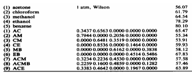
Finally, this problem was also solved by the late Prof. Floudas and co-workers using GAMS: see Chapter14 at: http://titan.princeton.edu/TestProblems/

We benchmark our results, summarized in the Table below, against data generated by a Matlab bifurcation code written by several people at the CHE department of MIT including the late Prof. Swan.

Results of the bifurcation analysis

This system has 9 azeotropes (6 binary azeotropes + 2 ternary azeotropes + 1 quaternary azeotrope).

# | x1 | x2 | x3 | x4 | x5 | T[°C]
────────────────────────────────
pure components:
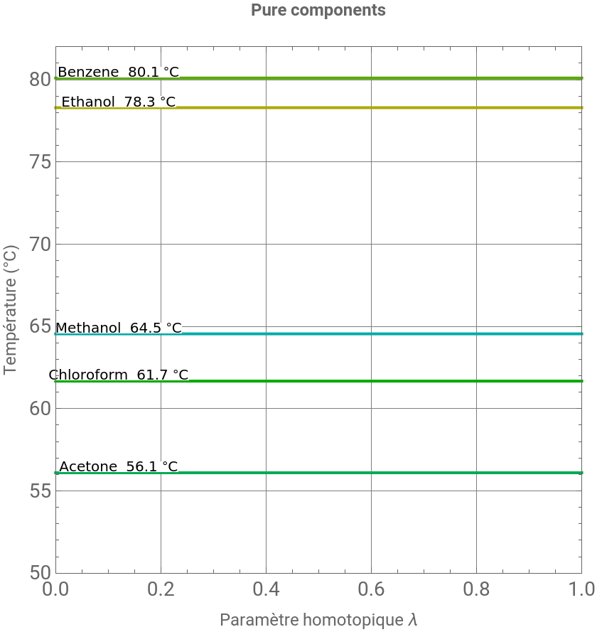
1 | 0.000 | 0.000 | 0.000 | 1.000 | 0.000 | 56.101
2 | 0.000 | 0.000 | 1.000 | 0.000 | 0.000 | 61.673
3 | 0.000 | 0.000 | 0.000 | 0.000 | 1.000 | 64.548
4 | 1.000 | 0.000 | 0.000 | 0.000 | 0.000 | 78.298
5 | 0.000 | 1.000 | 0.000 | 0.000 | 0.000 | 80.100

azeotropes:
6 | 0.000 | 0.000 | 0.655 | 0.000 | 0.345 | 53.896
7 | 0.000 | 0.000 | 0.000 | 0.792 | 0.208 | 55.394
8 | 0.000 | 0.050 | 0.205 | 0.295 | 0.450 | 57.361
9 | 0.000 | 0.000 | 0.225 | 0.338 | 0.437 | 57.368
10 | 0.000 | 0.377 | 0.000 | 0.000 | 0.623 | 58.288
11 | 0.142 | 0.000 | 0.858 | 0.000 | 0.000 | 59.712
12 | 0.179 | 0.000 | 0.482 | 0.340 | 0.000 | 63.285
13 | 0.000 | 0.000 | 0.663 | 0.337 | 0.000 | 64.553
14 | 0.463 | 0.537 | 0.000 | 0.000 | 0.000 | 68.211

Bifurcation Diagram

Doherty’s Homotopy Method (see Ref. 1)

ClearAll["Global`*"];

CONSTANTS

Total pressure

Ptot=760.0;

Universal gas constant

Rcal=1.9872041;

components={"Ethanol","Benzene","Chloroform","Acetone","Methanol"};abbrev={"Eth","Ben","Chl","Ace","Met"};

Antoine Equation

antoineParams={{8.11220,1592.864,226.184},{6.90565,1211.033,220.790},{6.93790,1171.173,227.000},{7.11714,1210.595,229.664},{8.08097,1582.271,239.726}};antoine[T_]:=Module[{Tc},Tc=T-273.15;10^(antoineParams[[All,1]]-antoineParams[[All,2]]/(antoineParams[[All,3]]+Tc))];

Wilson Model

V={58.68,89.41,80.67,73.93,40.73};AWilson={{0.0000,1239.9838,1559.2691,204.3217,-52.1274},{243.6327,0.0000,-3.1540,-429.2086,199.4167},{-352.7970,-96.5034,0.0000,-409.2236,-374.6921},{332.6937,5321.0769,6.1954,0.0000,-121.2515},{-52.3690,1629.3018,1818.2748,547.6712,0.0000}};lambdaWilson[T_]:=Table[If[i==j,1.0,(V[[j]]/V[[i]])*Exp[-AWilson[[i,j]]/(Rcal*T)]],{i,5},{j,5}];wilsonGamma[x_,T_]:=Module[{lam,S,lng},lam=lambdaWilson[T];S=lam.x;lng=Table[-Log[S[[k]]]+1-Sum[x[[i]]*lam[[i,k]]/S[[i]],{i,5}],{k,5}];Exp[lng]];

Pure components boiling temperatures

findTbp[i_]:=T/.FindRoot[antoine[T][[i]]-Ptot==0,{T,330}];Tbps=Table[findTbp[i],{i,5}];TbpsC=Tbps-273.15;

Homotopy Equations

doherty[v_,la_]:=Module[{x4,x5,x,T,psat,gam,K,f},x4=v[[1;;4]];x5=Max[1-Total[x4],10^-12];x=Join[x4,{x5}];x=x/Total[x];T=v[[5]];If[T<300||T>430,Return[ConstantArray[10^6,5]]];psat=antoine[T];gam=wilsonGamma[x,T];(*Correctthermodynamichomotopy*)K=(gam^la)*psat/Ptot;f=ConstantArray[0,5];Do[f[[i]]=x[[i]]*(K[[i]]-1),{i,4}];f[[5]]=K.x-1;f];

Initial guesses

initialGuesses={{0.463,0.537,0.000,0.000,341.4},{0.000,0.000,0.655,0.000,327.0},{0.000,0.000,0.663,0.337,337.7},{0.142,0.000,0.858,0.000,333.0},{0.000,0.000,0.000,0.792,328.5},{0.000,0.377,0.000,0.000,331.4},{0.000,0.000,0.230,0.330,330.5},{0.179,0.000,0.482,0.340,336.4},{0.001,0.050,0.204,0.294,330.5}};

Azeotropes

azeotropes={};Do[sol=Quiet@FindRoot[doherty[{x1,x2,x3,x4,T},1]=={0,0,0,0,0},{{x1,ig[[1]]},{x2,ig[[2]]},{x3,ig[[3]]},{x4,ig[[4]]},{T,ig[[5]]}},MaxIterations->500];xs={x1,x2,x3,x4}/.sol;x5=Max[1-Total[xs],0];xx=Join[xs,{x5}];xx=xx/Total[xx];temp=T/.sol;If[Max[xx]<0.99,AppendTo[azeotropes,<|"x"->xx,"T"->temp-273.15,"v"->({x1,x2,x3,x4,T}/.sol)|>]],{ig,initialGuesses}];azeotropes=DeleteDuplicates[azeotropes,Norm[#1["x"]-#2["x"]]<10^-3&];

Continuation

branches={};lambdaValues=N@Join[Range[0,0.8,0.02],Range[0.8,0.95,0.005],Range[0.95,1,0.001]];Do[v=az["v"];curve={};Do[sol=Quiet@FindRoot[doherty[{x1,x2,x3,x4,T},la]=={0,0,0,0,0},{{x1,v[[1]]},{x2,v[[2]]},{x3,v[[3]]},{x4,v[[4]]},{T,v[[5]]}},MaxIterations->300];v=({x1,x2,x3,x4,T}/.sol);AppendTo[curve,{la,v[[5]]-273.15}],{la,Reverse@lambdaValues}];active=Flatten@Position[az["x"],_?(#>0.04&)];AppendTo[branches,<|"curve"->curve,"active"->active,"n"->Length[active],"T1"->az["T"]|>],{az,azeotropes}];

Colors

pureColors=Table[Darker@Hue[i/12],{i,2,6}];branchColors=Table[Darker@Hue[i/12],{i,2,11}];

Pure lines

pureLines=Table[{pureColors[[k]],Thick,Line[{{0,TbpsC[[k]]},{1,TbpsC[[k]]}}]},{k,5}];

Branch graphics

branchGraphics=Table[Module[{curve,col,style,n},curve=br["curve"];n=br["n"];col=branchColors[[Mod[i-1,Length[branchColors]]+1]];style=Which[n==2,Directive[col,Dashed,Thick],n==3,Directive[col,Dashed,Thick],n>=4,Directive[col,Dashed,Thick]];{style,Line[curve]}],{i,Length[branches]},{br,{branches[[i]]}}];

Pure component labels

pureLabels=Table[Text[Style[components[[k]]<>" "<>ToString@NumberForm[TbpsC[[k]],{4,1}]<>" °C",10,Black,Background->White],{0.12,TbpsC[[k]]+.35}],{k,5}];

Pure components lines

p=Show[Graphics[{pureLines,pureLabels}],Frame->True,FrameLabel->{Style["Paramètre homotopique λ",12],Style["Température (°C)",12]},LabelStyle->Directive[14],PlotRange->{{0.0,1.},{50,82}},GridLines->Automatic,ImageSize->420,AspectRatio->1,PlotLabel->Style["Pure components\n",12,Bold]]

Out[]=

References

[1] Z.T. Fidkowski, M.F. Malone, M.F. Doherty, Computing azeotropes in multicomponent mixtures, Computers & Chemical Engineering, Volume 17, Issue 12, 1993, Pages 1141-1155, https://doi.org/10.1016/0098-1354(93)80095-5

CITE THIS NOTEBOOK

Systematic determination of the azeotropes of a pentanary system by bifurcation
by Samar Jebali, Oumaima ben saad, Ons Zarraa, Eya kefi, Yassmine ben hamouda, Housam Binous, and Ahmed Bellagi
Wolfram Community, STAFF PICKS, May 24, 2026
https://community.wolfram.com/groups/-/m/t/3721524