Reinventing the SVD decomposition from cartography
“Rotate-Squish-Rotate” matrix decomposition
by Rauan Kaldybaev
“Rotate-Squish-Rotate” matrix decomposition
by Rauan Kaldybaev
The current essay reinvents the concept of the singular value decomposition of a matrix from the discussion of the Tissot indicatrix. A generic matrix can be viewed as a linear transformation on the 2-dimensional space. Correspondingly, one way to describe a matrix is by examining the ellipse that results from acting by this matrix on the unit circle. Matrices with positive determinants can be written as a product of several terms, each of which takes care of one of the properties of the ellipse, namely: area, eccentricity, orientation of the major axis, and the position of the points within the ellipse. After inventing the rotate-squish-rotate decomposition, I have observed that it turns out to be equivalent to the SVD decomposition. This of course reduces the novelty of the essay, though the approach used here is still quite interesting. One possible application (and the original inspiration) of the RSR decomposition is cartography, where it can be used to measure the distortion of a map projection.
22
22
Introducing the ellipse plot of a matrix; the Tissot indicatrix
Introducing the ellipse plot of a matrix; the Tissot indicatrix
A 2x2 matrix describes a linear transformation on the 2-dimensional space. A matrix can shorten, stretch, or rotate objects. The action of a matrix can be visualized using what I call its ellipse plot, which is basically how the matrix does to the unit circle. To draw the ellipse plot of a matrix , one just needs to take all the points on the unit circle and act on them by . Mathematically, the unit circle can be parametrizes as
for , and the ellipse plot of is then the parametric plot of . The ellipse plot of the identity matrix is just the original unit circle; matrices with a large positive determinant make ellipses with a large area, and singular matrices generate ellipses with zero area, or basically straight lines. Here are examples of the three cases:
M
M
Cos[α] |
Sin[α] |
α∈[0,2π]
M
M
Cos[α] |
Sin[α] |
In[]:=
ParametricPlot[#.{Cos[α],Sin[α]},{α,0,2π},PlotLabel->Row[{"Area = ",Det[#]}]]&/@
,
,
1 | 0 |
0 | 1 |
4 | 3 |
-4 | 2 |
1 | 2 |
2 | 4 |
Out[]=
,
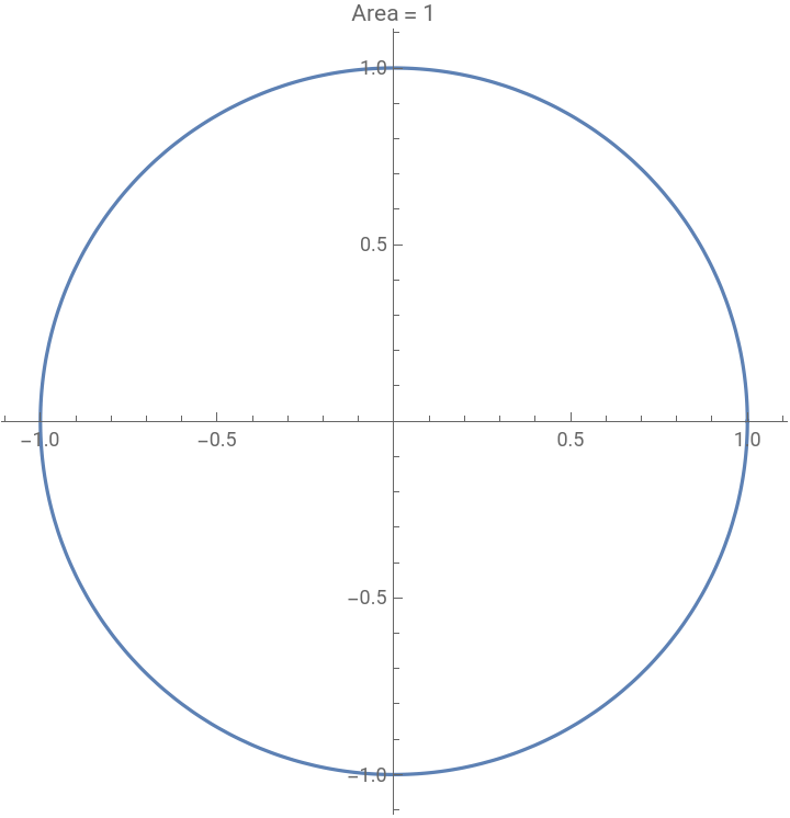
,
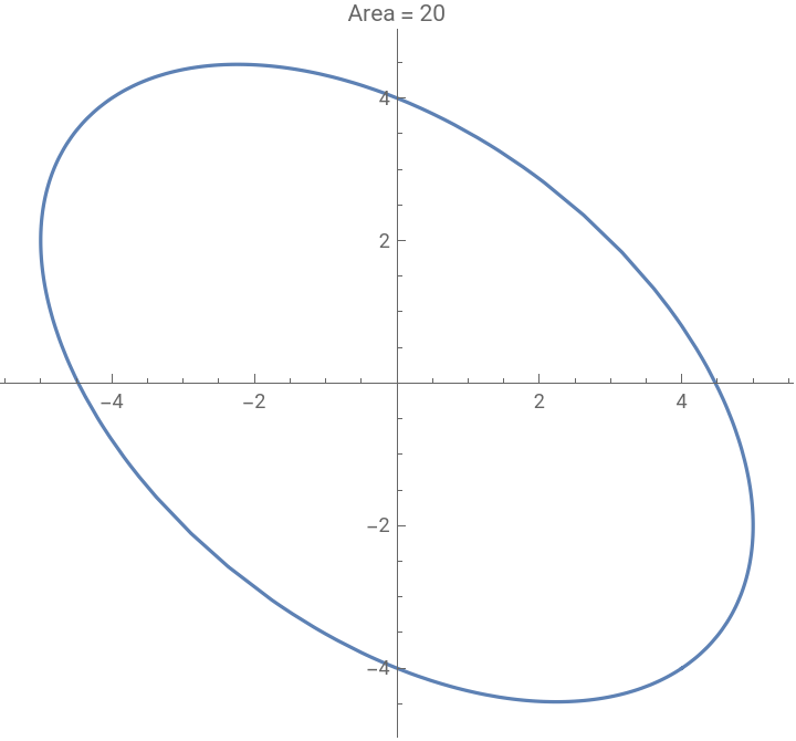
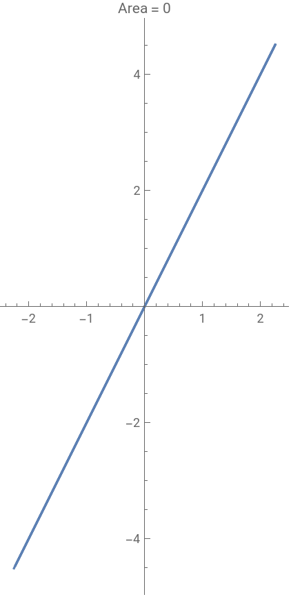
To make the plot more informative, one can also color the ellipse by . This way, the plot can also keep track of rotation. Here is the comparison of the ellipse plot of an identity matrix to that of a 45 degree rotation matrix. You can see that the ellipse plot for the rotation matrix is rotated by 45 degrees:
α
In[]:=
ClearAll[matrixEllipsePlot];matrixEllipsePlot[M_, options___] := ParametricPlotM.
, {α, 0, 2π}, options, ColorFunction -> Function[{x, y, α}, Hue[α]]
Cos[α] |
Sin[α] |
In[]:=
{matrixEllipsePlot[IdentityMatrix[2]],matrixEllipsePlot[RotationMatrix[π/4]]}
Out[]=
,
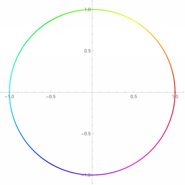
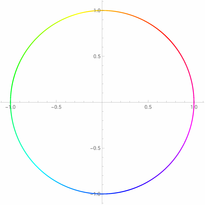
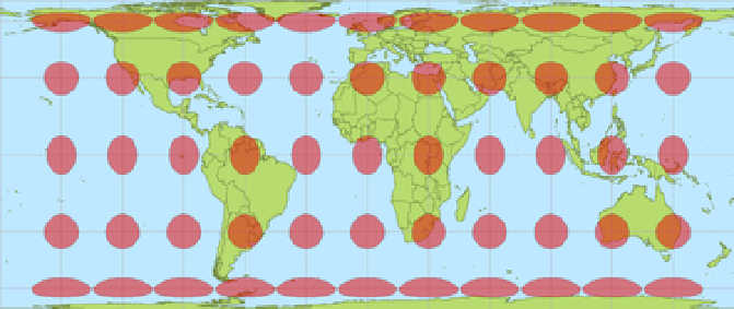
A version of the ellipse plot is used in cartography, where it is known as the Tissot indicatrix. It is used to evaluate the degree by which map projections distort the look of the Earth’s surface. Although map projections are not linear, they can be linearized around fixed points, and the Tissot indicatrix is basically the ellipse plot of the Jacobian matrix from the coordinates parametrizing the Earth’s surface to coordinates on the (paper) map. Actually, the inspiration for this essay came to me from looking at the Tissot indicatrix. Here is an example of the Tissot indicatrix (image from Wikipedia):
It seems like the ellipse plot of a matrix summarizes all the information about it in a neat and very visual way. This is the idea behind the rotate-squish-rotate decomposition.
Introducing the Rotate-Squish-Rotate decomposition
Introducing the Rotate-Squish-Rotate decomposition
An ellipse can be characterized by three parameters: its area, the ratio of its major and minor axes, and the angle between the major axis and the x axis. The ellipse plot of a matrix is also an ellipse. To “fabricate” a matrix to produce an ellipse of given parameters, we can just use the formula , where is a scalar, is a rotation matrix by angle , and is a matrix of hyperbolic rotation by . takes care of the determinant, makes the ellipse have the right eccentricity, and rotates the ellipse (because and both have a determinant of 1, they don’t interfere with ). But this cannot be sufficient to express all the information about a 2x2 matrix because the latter has four numbers in it and an ellipse has just three parameters. In other words, two different matrices can in fact produce an ellipse of the same shape - for example, the identity matrix and a rotation matrix both produce a unit circle. And this is a clue: the missing parameter is rotation. In the formula, the point always lies either on the major or the minor axis of the ellipse because is diagonal. But if another rotation matrix is added in front, it can be arranged that any point lie on the major axis. So, the final formula is:
M=kR[θ]H[ψ]
k
R[θ]=
Cos[θ] | -Sin[θ] |
Sin[θ] | Cos[θ] |
θ
H[ψ]=
Exp[ψ] | 0 |
0 | Exp[-ψ] |
ψ
k
H
R
R
H
k
M=kR[θ]H[ψ]
(1,0)
H[ψ]=
Exp[ψ] | 0 |
0 | Exp[-ψ] |
M=kR[θ]H[ψ]R[ϕ]
(
1
) Applying to the unit circle first rotates it, then squishes, and then rotates again (and also scales, but that’s trivial) - hence the name rotate-squish-rotate. Here is a picture illustrating how this works:
kR[θ]H[ψ]R[ϕ]
In[]:=
BlockM=
,k,θ,ψ,ϕ,dec,dec=rsrDecomposition[M];k=dec[[1]];θ=dec[[2]];ψ=dec[[3]];ϕ=dec[[4]];matrixEllipsePlot[#[[2]],PlotLabel->#[[1]],PlotRange->{{-2.5,2.5},{-3.5,3.5}}]&/@{{"Unit circle (do nothing)",matrixFromRSR[1,0,0,0,False]},{"Rotate, R[ϕ]",matrixFromRSR[1,0,0,ϕ,False]},{"Squish, H[ψ]",matrixFromRSR[1,0,ψ,ϕ,False]},{"Rotate, R[θ]",matrixFromRSR[1,θ,ψ,ϕ,False]},{"Scale, k",matrixFromRSR[k,θ,ψ,ϕ,False]}}
1 | -2 |
1 | 3 |
Out[]=
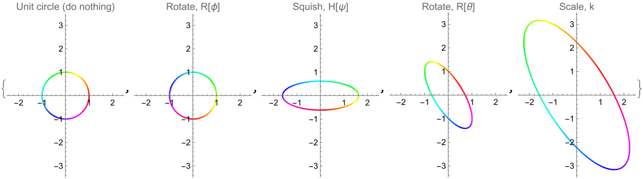
The numbers are not hard to find. First of all, and have determinant 1, so . By writing for a point on the unit circle, for a point on the ellipse plot, and using trig formulas to simplify y, we can find the lengths of the major and minor semiaxes of the ellipse. Because rotations don’t deform the ellipse and just rotate it, the proportions of the ellipse are completely determined by ; namely, the ratio of the major axis to the minor axis is given by . From here, one can find . To find , one can use the fact that (for positive ) the matrix takes the point to lie on the ellipse’s major axis, so whatever point was moved to by ends up lying on the major axis of the ellipse; this happens to the point with . On the other hand, we can study y to determine for what value of is y maximal - in other words, what corresponds to a point on the major axis of the ellipse. Combining that information, we can find . Lastly, is just the angle between the ellipse’s major axis and the x axis. Here are the formulas:
k,θ,ψ,ϕ
R
H
k=
Det[M]
x=
Cos[α] |
Sin[α] |
y=Mx
T
y
ψ
Exp[2ψ]
ψ
ϕ
ψ
H
(1,0)
(1,0)
R[ϕ]
α=-ϕ
T
y
α
T
y
α
ϕ
θ
k=Cos[]+Sin[],Cos[]+Sin[]]ψ=Logϕ=-
Det[M]
θ=ArcTan[m
11
α
m
m
12
α
m
m
21
α
m
m
22
α
m
1
4
w+s
w-s
α
m
(
2
) where , , , , , and =ArcTan[u,v]; is the value of which corresponds to lying on the major axis of the ellipse. The RSR decomposition of a 2 by 2 matrix is not unique. The most obvious way is that could be added to either or , and this wouldn’t make any difference. Also, replacing by has no effect either because is equivalent to - this is because for , stretches the direction and shortens the direction, and for , it does exactly the opposite; a couple of rotations can effectively turn into . Here is how the formula (2) can be used on the matrix :
A≡M
T
M
u≡-
a
11
a
22
v≡+
a
12
a
21
w≡+
a
11
a
22
s≡+
2
u
2
v
α
m
1
2
α
m
α
M
Cos[α] |
Sin[α] |
2π
θ
ϕ
θ,ψ,ϕ
θ-π/2,-ψ,ϕ+π/2
H[ψ]
R[-π/2]H[-ψ]R[π/2]
ψ>0
H[ψ]
x
y
ψ<0
H[ψ]
H[-ψ]
-9 | -1 |
5 | -5 |
In[]:=
N@rsrDecomposition
-9 | -1 |
5 | -5 |
Out[]=
{7.07107,2.54645,0.390035,0.190253,False}
And here is the reconstructed matrix:
In[]:=
MatrixForm@N[7.0710678118654755`RotationMatrix[2.5464476787485273`].hyperbolicRotationMatrix[0.39003531977071526`].RotationMatrix[0.19025318855618245`]]
Out[]//MatrixForm=
-9. | -1. |
5. | -5. |
We’ve got back to the original matrix. One thing you might have noticed is that in addition to the four numbers, the output of the function rsrDecomposition (code below) also included False. This has to do with the fact that the formula (2) is actually only valid for matrices with positive determinants. If the determinant is zero, then the ellipse plot is just a line, which corresponds to infinite ; attempting to use the formula (2) leads to an undefined situation of the type . When the determinant is negative, the formula doesn’t work because a matrix with a negative determinant “reverses” shapes, which cannot be achieved through rotations, hyperbolic rotations, or scaling. But a matrix with a negative determinant can be made into a matrix with a positive determinant by changing the sign of one of the rows as . RSR can then be done on the modified matrix, and to get the original matrix , we just need to do - this is because , and =I. One other special case that needs addressing is when the ellipse plot of a matrix is a circle, which in some sense means that there isn’t a single definite major axis. In that case, trying to find the value of for which the point lies on the major axis is a futile problem because is the same for all , and so any value of would do. Because every value is fine, in this situation one way to go is to just pick =0. Here is the code for rsrDecomposition:
ψ
Log[0]
M
M
1 | 0 |
0 | -1 |
M
k
R[θ]H[ψ]R[ϕ]
1 | 0 |
0 | -1 |
kR[θ]H[ψ]R[ϕ]=
M
1 | 0 |
0 | -1 |
2
1 | 0 |
0 | -1 |
α
M
Cos[α] |
Sin[α] |
M
Cos[α] |
Sin[α] |
α
α
α
m
Meaning and possible applications of the RSR decomposition
Meaning and possible applications of the RSR decomposition