Over 200 subatomic particles have been detected by scientists, most of which are highly unstable. Additionally, subatomic particles have many underlying properties that determine their quantum behavior, such as spin, quark content, and Compton wavelength. These properties are crucial for understanding how they interact and decay in various conditions. This first half of this project aims to explore particle decay chains primarily via constructing directed graphs and hypergraphs of decay product groups of for all particles in Wolfram’s ParticleData. The second half of this project investigates the contributions of particle properties in determining particle classifications on Regge trajectories.
Introduction
Particle Decay
Particle Decay
Subatomic particles transform into lighter, more stable particles, often through a series of intermediate steps in a decay chain. Each step follows specific conservation laws and can involve multiple decay modes with varying probabilities, called branching ratios. Clear, well-designed visualizations of these decay pathways are helpful for mapping these processes, simplifying tracing particle transformations to better identify shared decay products and uncover underlying patterns in particle behavior.
Regge Trajectories
Regge Trajectories
Regge trajectories are a consequence of Regge theory, originally developed by Tullio Regge in 1959. Empirically, it was found that some particles lie on a similar “trajectory” in a plot of vs. quantum spin. In theory, particles with the same internal quantum numbers will lie on the same linear Regge trajectory, suggesting they are related by the same underlying force or structure—typically modeled as rotating strings or resonances of a common system.
2
mass
The Quantum Schrödinger Equation
The Quantum Schrödinger Equation
The Schrödinger equation is a foundational equation in quantum mechanics that describes how the quantum state of a particle evolves over time. It governs the behavior of wavefunctions, which encode the probabilities of a particle’s position, momentum, etc. Solving the Schrödinger equation for specific potentials yields quantized energy levels in the form of energy eigenvalues, which we will use to validate our Regge trajectories.
iℏΨ(x,t)=+V(x,t)Ψ(x,t)
∂
∂t
-
2
ℏ
2m
2
∂
∂
2
x
Time-dependent Schrödinger equation.
Part I - Decay Chain Plots
The first half of this project involves creating graphs of particle decay chains for all particles with applicable information in the Wolfram library. Firstly, we had to filter through the dataset to remove any instances with missing or incomplete information, either for resulting particles or their respective branching ratios. We were then able to create flowchart-type plots for remaining particles with all the necessary information (approximately 200). The vertices are labelled with the corresponding particle, and the edges similarly depict the normalized branching ratios.
Data Processing
Data Processing
Filter through ParticeList and removes empty values, missing particle decays, and missing branching ratios. layerAll represents the cleaned association lists.
particleList=EntityList["Particle"];decayModeList=AssociationMap[#["DecayModes"]&,particleList];nonEmpty=Select[decayModeList,Length[#]!=0&];nonMissingFirstLevel=Select[nonEmpty,!MissingQ[#]&];filteredRows=Select[nonMissingFirstLevel,AnyTrue[Values[#],!MissingQ[#]&]&];finalParticleList=filteredRows/.(x_->Missing["Observed"]):>(x->0);
In[]:=
Dataset[RandomSample[finalParticleList,5]]
Out[]=
|
Decay Graphs
Decay Graphs
Construct both single-layer simple decay graphs and hypergraphs of particle decay modes to visualize their paths of evolution.
Single-Layer Simple Decay Graphs
Single-Layer Simple Decay Graphs
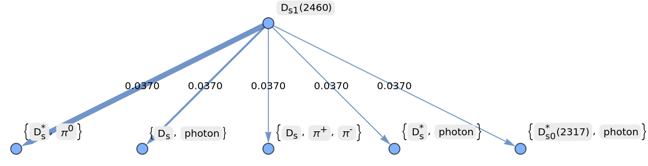
Simple directed single-layer decay graphs based on association data of particle decay modes and with widths proportional to normalized branching ratios.
In[]:=
Clear[makeDecayGraphs];makeDecayGraphs[filteredRows_,particle_]:=Module[{row,outerKey,innerKeys,edges,brs,styles,weights},row=filteredRows[particle];(*outerKey=Keys[row];*)innerKeys=Keys[row];edges=Flatten[{particle->#}&/@innerKeys,1];brs=Values[row];styles=Map[{Thickness[#/100]}&,Rescale[brs]];Graph[edges,VertexLabels->"Name",EdgeWeight->Thread[edges->weights],EdgeStyle->Thread[edges->styles],EdgeLabels->brs]]
Sample decay graph for (2460) particle. Note the branching ratios won’t always sum to 1 due to missing or incomplete data.
D
s1
In[]:=
makeDecayGraphsfilteredRows,
Out[]=
Hypergraph of all Particle Decays
Hypergraph of all Particle Decays
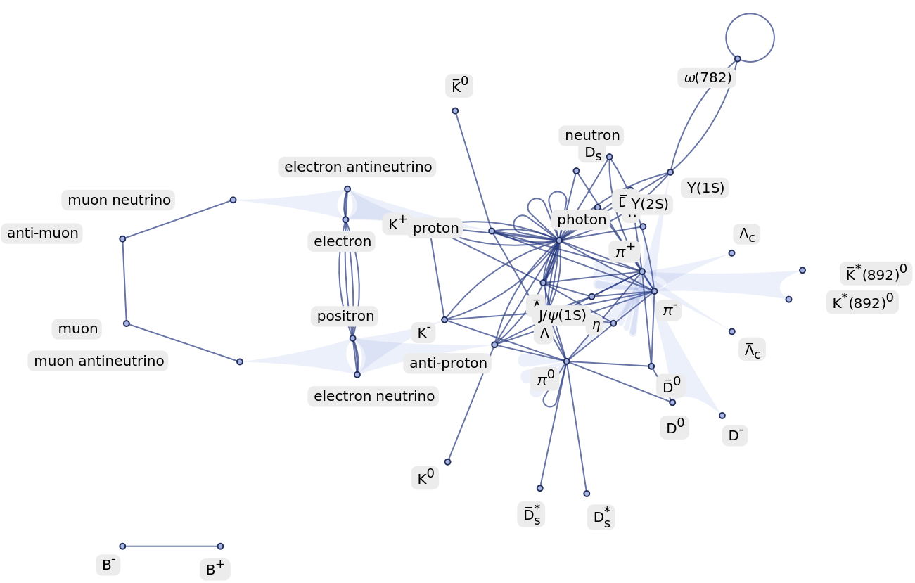
Hypergraph of all particles’ interconnected cyclical decay chains.
Import and install the Wolfram Hypergraph paclet.
In[]:=
PacletInstall["WolframInstitute/Hypergraph"];Needs["WolframInstitute`Hypergraph`"];
In[]:=
hyperedges=Quiet[Flatten[Table[With[{parent=Keys[row][[1]],decayTable=Values[row][[1]]},KeyValueMap[(#1->#2)&,AssociationThread[ConstantArray[parent,Length[Keys[decayTable]]],Keys[decayTable]]]],{row,filteredRows}],1]];Hypergraph[hyperedges,VertexLabels->"Name"]
Out[]=
Hypergraph of Individual Particle Decays
Hypergraph of Individual Particle Decays
We specifically chose to utilize a hypergraph in order to convey the clustering of particles in different decay groups. This proved difficult due to the multiplicity of most decay particles, overlapping between different decay groups. This required the use of multi-layer particle tagging in order to correctly differentiate them between product groups, especially in the pseudo-recursive section, while simultaneously preventing incorrect association from appearing within the same group.
Creating a particle decay hypergraph.
In[]:=
particleDecayToHypergraph[parentParticle_,decayModes_Association]:=Module[{hyperedges,vertices,taggedParticles,decayCounter},decayCounter=0;hyperedges={};taggedParticles=<||>;KeyValueMap[Function[{decayProducts,branchingRatio},Module[{taggedProducts},decayCounter++;taggedProducts=Table["tag$"<>ToString[decayCounter]<>"$"<>ToString[i],{i,Length[decayProducts]}];AppendTo[hyperedges,Prepend[taggedProducts,"parent"]];taggedParticles[decayCounter]=<|"products"->decayProducts,"tagged"->taggedProducts,"ratio"->branchingRatio|>;]],decayModes];vertices=DeleteDuplicates[Flatten[hyperedges]];<|"Hyperedges"->hyperedges,"Vertices"->vertices,"ParentParticle"->parentParticle,"TaggedParticles"->taggedParticles,"DecayModeCount"->decayCounter|>];
In[]:=
visualizeParticleDecay[result_Association]:=Module[{hyperedges,vertices,parentParticle,vertexLabels,taggedParticles},hyperedges=result["Hyperedges"];vertices=result["Vertices"];parentParticle=result["ParentParticle"];taggedParticles=result["TaggedParticles"];vertexLabels=Join[{"parent"->parentParticle},Flatten[Table[MapThread[Rule,{taggedParticles[i]["tagged"],taggedParticles[i]["products"]}],{i,result["DecayModeCount"]}]]];ResourceFunction["HypergraphPlot"][hyperedges,VertexLabels->vertexLabels,"SubsetBoundary"->Automatic,"BaseLayout"->"RadialEmbedding",VertexSize->0.03]];
In[]:=
result=visualizeParticleDecayparticleDecayToHypergraph,["DecayModes"]
Hypergraph of Multi-Step Particle Decays
Hypergraph of Multi-Step Particle Decays
Example of a hypergraph of particle decays which takes an input particle and creates layered branches of consecutive decays up to the second level. In this example, we are displaying the Omega to Lambda decay chain. Using the hypergraph visualization, we are able to better determine the groups in which each of the particles decay in, and the chain reaction effect going from Omega to Lambda and beyond.
Part II - Investigation of Properties Correlated with Regge Trajectories
Mass Squared vs. Spin Plot for All Particles
Mass Squared vs. Spin Plot for All Particles
A Regge scatter plot (mass squared vs. spin) for all available and complete particles in the Wolfram library.
Regge Trajectories for Different Particle Families
Regge Trajectories for Different Particle Families
If particles on a coordinate plane of mass squared vs. spin yields a linear line of best fit (i.e. a linear Regge trajectory), that would imply these particles are likely part of the same family of hadronic resonances. Notably, as the spin of the particles increases, their mass squared increases proportionally, consistent with models where particles are bound by a linear potential, revealing underlying patterns governing the properties of these particles.
Function to select all the appropriate/applicable particles for any given selection criteria.
Function to select particles near the Regge trajectory with a similar quark content.
Function select particles within a given residual distance from the line of best fit (Regge trajectory); used for later research.
Expanding Selections of Particles Collinear on a Regge Trajectory
Expanding Selections of Particles Collinear on a Regge Trajectory
Given previously discovered classes of particles that we already know share a Regge trajectory, we aim to investigate if there exists other particles across the dataset which are incorrectly sorted into their particle family and could potentially lie on the same Regge trajectory. Particles on the same Regge trajectory should share a G-parity and isospin value, and have a linear association between their spin and mass-squared values. For simplicity, the internal quantum numbers can be inferred via constituent quarks as opposed to querying for individual properties.
ρ Mesons
ρ Mesons
Investigation of potentially missing particles on the ρ Meson Regge trajectory by determining the equation for the line of best fit, and then selecting particles with a residual from the line smaller than 0.1 which also share the same quantum numbers.
Fit a linear model to an already well-known Regge trajectory.
Demonstrating that all of these particles have the same quark content, isospin, and G-parity.
Filter results to isolate other particles with the same quark content.
Find particles that are very close or on our linear potential fit.
We can find which particles lie close to the linear fit, and also have the same quark content as our ρ mesons.
Interestingly, we discovered that these two particles do not actually share the same isospin as the rest of the ρ meson particles, suggesting they are not part of the exact same Regge trajectory. However, it is possible that they lie on close, parallel trajectories.
Δ Baryons
Δ Baryons
Investigation of potentially missing particles on the Δ Baryon Regge trajectory by determining the equation for the line of best fit, and then selecting particles with a residual from the line smaller than 0.1 which also share the same quantum numbers.
Fit a linear model to a previous discovered Regge trajectory.
Show that all of these particles have the same quark content, isospin, and G-parity.
Find other particles with the same quark content.
Find particles that are very close to our linear model fit.
We can find which particles lie close to the linear fit, and also have the same quark content as our Δ baryons.
f Mesons
f Mesons
Investigation of potentially missing particles on the f meson Regge trajectory by determining the equation for the line of best fit, and then selecting particles with a residual from the line smaller than 0.1 which also share the same quantum numbers.
Fit a linear model to a well-known Regge trajectory.
Show that all of these particles have the same quark content, isospin, and G-parity.
Find other particles with the same quark content.
Find particles that are very close to our linear model fit.
We can find which particles lie close to the linear fit, and also have the same quark content as our f mesons:
Theoretical vs. Experimental Trajectories via Schrödinger’s Equation for ρ Mesons
Theoretical vs. Experimental Trajectories via Schrödinger’s Equation for ρ Mesons
Information to solve the Schrödinger equation, including reduced mass of quark-antiquark system and string tension for a linear potential system.
Schrödinger equation operator (includes units).
We’re using the Schrödinger equation here to compute theoretical mass spectra for hadronic systems under a chosen potential (linear), treating the mesons as bound states of quarks. By solving the equation for different angular momentum values from energy eigenvalues, we generate predicted values of mass squared that can be plotted against spin. This gives us a theoretical Regge trajectory, which we can then compare to experimental particle data. If the Schrödinger-based predictions produce a linear or nearly linear trajectory matching the experimental one, it provides evidence that the underlying potential and quantum model accurately describe the confinement dynamics in mesons.
Theoretical vs. Experimental Trajectories via Schrödinger’s Equation for Δ Baryons
Theoretical vs. Experimental Trajectories via Schrödinger’s Equation for Δ Baryons
Schrödinger approximation for delta baryons.
Closing
Conclusion
Conclusion
In the first half of my project, I successfully created decay chain plots for all particles in the Wolfram database. Not only did I create an interconnected plot of all particles showing their cyclical decay relationships, I also created flat directed decay graphs for each individual particle. I also implemented hypergraphs to better visualize particle decay within subgroups of products, including multi-layer decays. The effective visualizations of these decay pathways are helpful for mapping these processes, simplifying tracing particle transformations to better identify shared decay products and uncover underlying patterns in particle behavior.
In the second half, I investigated subatomic properties and quantum numbers (inferred from non-elementary particles’ quark contents) and their relationship to Regge trajectories (plots of particle mass-squared vs. spin). We were reliably informed that due to potential misnomers of particles, we could hypothesize to find additional particles in the gaps of our linear potential trajectories with the missing spin values. Within the three particle families analyzed, we did not find external additions to the Regge trajectories for ρ mesons, but potentially for Δ baryons.
In the second half, I investigated subatomic properties and quantum numbers (inferred from non-elementary particles’ quark contents) and their relationship to Regge trajectories (plots of particle mass-squared vs. spin). We were reliably informed that due to potential misnomers of particles, we could hypothesize to find additional particles in the gaps of our linear potential trajectories with the missing spin values. Within the three particle families analyzed, we did not find external additions to the Regge trajectories for ρ mesons, but potentially for Δ baryons.
Future Direction
Future Direction
In the future, I would like to further study particle decay patterns to better understand the causes of different branching ratios and probabilities of decay product outcomes. For example, I’d investigate how effective lifetimes and strangeness conservation of certain particles (in association with the force causing the decay) contribute to different outcomes. This would shed light on some of the missing branching ratios in the Wolfram database and gaps in our general knowledge, which are theoretically possible decays but occur very rarely or not at all. Furthermore, I’d like to validate the results of my Schrödinger approximation for different potentials (not just linear) and eventually move to the Dirac equation, which offers a relativistic approximation as opposed to the non-relativistic nature of the Schrödinger equation. Lastly, the layered decay hypergraphs are not fully autonomous; next steps would be to successfully implement a truly recursive hypergraph which iterates through every last layer.
References
References
Freedman, D. Z. (1964, May 11). Model for the nucleon and baryon Regge trajectories. Physical Review, 134(3B), B652. https://doi.org/10.1103/PhysRev.134.B652
Tang, A., & Norbury, J. W. (2000). Properties of Regge trajectories (preprint). arXiv. https://arxiv.org/pdf/hep-ph/0004078
Tang, A., & Norbury, J. W. (2000). Properties of Regge trajectories (preprint). arXiv. https://arxiv.org/pdf/hep-ph/0004078
Acknowledgements
Acknowledgements
I would like to extend my gratitude to my mentor Joseph Brennan for guiding and supporting me throughout this project with such insight, dedication, and *attention to detail*! I would also like to thank Stephen Wolfram and the WSRP program directors for providing the framework and direction of the project. Lastly, I would like to thank all the TAs, especially Sanay Nesargi and Alisa Zaitseva, and all my peers for their support and for making this program so memorable.
CITE THIS NOTEBOOK
CITE THIS NOTEBOOK
Visualizing particle decay chains and analyzing Regge trajectories
by Julia Gao
Wolfram Community, STAFF PICKS, July 10, 2025
https://community.wolfram.com/groups/-/m/t/3501714
by Julia Gao
Wolfram Community, STAFF PICKS, July 10, 2025
https://community.wolfram.com/groups/-/m/t/3501714