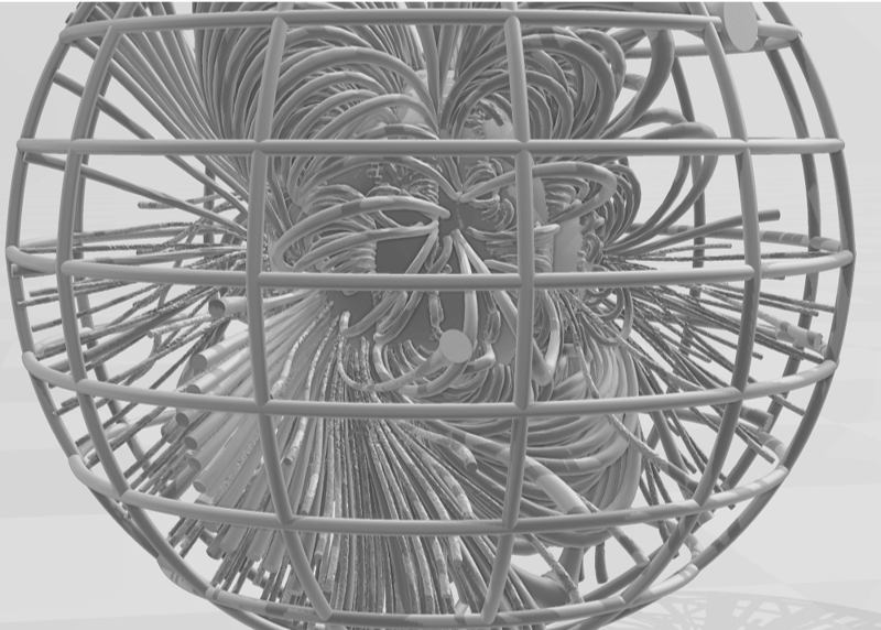
With this model the solar magnetic field lines and the magnetic field strengths are calculated hence the magnetic flux tubes can be generated. Its data is obtained from The WSA ( Wang-Sheeley-Arge ) model which is used to derive solar wind speed. The model uses photospheric magnetograms to calculate the coronal field. It is based on the idea that, far from the Sun, the speed of the solar wind depends on the path that the wind took as it passed through the lower corona. It models the coronal magnetic field which will be used to generate a 3D printing model of the sun.
NOTE: We have to use an older version of Mathematica , version 12.3.1 (2021), since the code to generate “Tube” is not compatible with V14 yet.
The WSA ( Wang-Sheeley-Arge ) model is used to derive solar wind speed. The model uses photospheric magnetograms to calculate the coronal field. It is based on the idea that, far from the Sun, the speed of the solar wind depends on the path that the wind took as it passed through the lower corona. It models the coronal magnetic field which will be used to generate a 3D printing model of the sun. With this model the magnetic field lines and the magnetic field strengths are calculated hence the magnetic flux tubes can be generated.
In[]:=
nuver=$VersionNumber
Out[]=
12.3
In[]:=
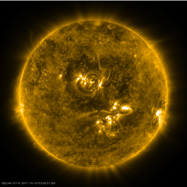
If[nuver>13,ResourceFunction["SolarImage",ResourceSystemBase->"https://www.wolframcloud.com/obj/resourcesystem/api/1.0"][DateObject[{2017,10,2}],11]](*11=SDOAIA193needMathematica14.1forthislineofcode.*)
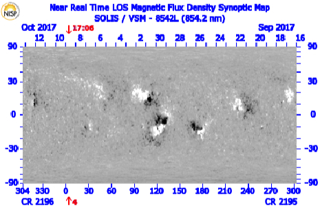
Potential field lines for the sun for the
Carrington Rotation: 2196 _304 09 Oct 2017 17:06 UT
Date files can be found here:
https://drive.google.com/drive/folders/1OHV5BuqZPA6ze-E3JuK9t5SsPPSyNpkD?usp=sharing
Carrington Rotation: 2196 _304 09 Oct 2017 17:06 UT
Date files can be found here:
https://drive.google.com/drive/folders/1OHV5BuqZPA6ze-E3JuK9t5SsPPSyNpkD?usp=sharing
In this Mathematica program the magnetic flux tubes are calculated which is an extension of a previous program
(see https://community.wolfram.com/groups/-/m/t/3319778).
Again this program was generated using the Community Coordinated Modeling Center - GSFC.
For a 3D printing model of the solar coronal, the model need enough lines around a few active regions to simulate the coronal images that might be made. The model needs field lines and magnetic field strength to show the overall structure over the full sphere. The magnetic flux tubes are generated with enough flux tubes to show the details of the total solar coronal structure. In the 3D print model the outer source surface (R=2.5 solar radius) is shown.
This Mathematica model will read each the lines x,y,z, and field strength at each point via spherical coordinates for both field coming from the solar surface and from the solar source surface.
Notes: from CCMC:
The WSA ( Wang-Sheeley-Arge ) model records fieldlines were provide in 3 separate files, all combined in a tar file.
1. tracing inward from the outer boundary of the Schatten current sheet (5Rsun) to the source surface (at2.5Rsun) in fs2/Data/WSA-6.2/WSA_WORKING/CCMC/QuickStart/CORONA/trace_scs_outtoin
2. continuing these fieldlines from the source surface to the solar surface, in
fs2/Data/WSA-6.2/WSA_WORKING/CCMC/QuickStart/CORONA/trace_pfss_outtoin
3. drawing fieldlines from the solar surface in
fs2/Data/WSA-6.2/WSA_WORKING/CCMC/QuickStart/CORONA/trace_pfss_intoout
The fits file headers give a comprehensive description of the data in each file.
The image in
fs2/Data/WSA-6.2/WSA_WORKING/CCMC/QuickStart/PLOTS/CORONA/wsa_202411051404R000_gong_1_6_4.png
shows you the standard WSA view of the solution so you can get an idea of the field complexity.
The coupling of the PFSS and Schatten CS give kinks in the field lines at their common boundary, which WSA tries to smooth out. CCMC suggested that it might be good to explore additional smoothing there when one is converting the files into the format for the 3D printer. Also, field lines in CCMC files use the default selection of starting points which is a set of uniformly spaced points on the outer sphere, with 180 in the azimuthal direction and 90 in the latitude direction, with an additional set of 180x3 lines drawn about the plane of the ecliptic.
The fits files in the Trace directories are given as tables. The primary data extension has a 6x300x16740 array.
If we use i,j,k to index the array, each k index represents a distinct field line, with <=300 points along a field line, and 6 data values at each field line point (phi coord, theta coord, radial coord, Bphi, Btheta, Bradial). Most field lines have less than 300 points so where there is a value of -999.99, that can be ignored. Field lines are drawn both inward (‘outtoin’) from the outer boundary of the current sheet component (at 5Rsun) to make sure lots of open field lines are included, and ‘intoout’ from the solar surface to make sure closed field region fieldlines are also drawn. There are 180 x (90 + 3) = 16740 fieldlines in both of the outtoin files. These 2 files need to be combined to complete the ‘outtoin’ fieldlines. The 180x90 set (k=t to 16200) start from an evenly spaced set of grid points on the sphere at 5Rsun. The extra 180x3 lines (k=16201 to 16740) of starting points (I believe) are started from a circle of 180 point around the plane of the ecliptic and +/- delta_theta either side of the plane of the ecliptic (not sure what delta_theta is set to).
For the intoout fits file, the data array has the same dimensions. The extra points, k=16201 to 16740, seem to be unused space.
In[]:=
(*Import["C:\\Users\\gag00\\OneDrive\\Desktop\\Solar3Dmodel\\FINALFinalEdition\\wsa62_quickstart_run.tar",*)
For reading the tar-file is on a Dell desktop using MS Windows 11, where one can right clicked on the .tar files and is able to extract all the files to file Tar Files which consisted of:
“C:\Users\gag00\OneDrive\Desktop\Tar Files\resize.list”
“C:\Users\gag00\OneDrive\Desktop\Tar Files\pregongz.list”
“C:\Users\gag00\OneDrive\Desktop\Tar Files\pre_out_list.txt”
“C:\Users\gag00\OneDrive\Desktop\Tar Files\mrzql241105t1404c2290_040.fits.gz”
“C:\Users\gag00\OneDrive\Desktop\Tar Files\int_out_list.txt”
“C:\Users\gag00\OneDrive\Desktop\Tar Files\int_202411051404_gongz.fits”
“C:\Users\gag00\OneDrive\Desktop\Tar Files\gongz_date_list.txt”
“C:\Users\gag00\OneDrive\Desktop\Tar Files\202411051404R000_trace_scs_outtoin_tracing.fits”
“C:\Users\gag00\OneDrive\Desktop\Tar Files\202411051404R000_trace_pfss_outtoin_tracing.fits”
“C:\Users\gag00\OneDrive\Desktop\Tar Files\202411051404R000_trace_pfss_intoout_tracing.fits”
“C:\Users\gag00\OneDrive\Desktop\Tar Files\wsa_202411051404R000_gongz.fits”
“C:\Users\gag00\OneDrive\Desktop\Tar Files\wsa_202411051404R000_gong_1_6_4.png”
“C:\Users\gag00\OneDrive\Desktop\Tar Files\syn_202411051404_gongz.fits”
“C:\Users\gag00\OneDrive\Desktop\Tar Files\sbe_202411051404_gongz.fits”
These files were placed in folder named ”C:\\Users\\gag00\\OneDrive\\Desktop\\Tar Files”
For importing these files into Mathematica see the online notes:
https://www.wolfram.com/language/12/data-import-and-export/fits-updates.html
In[]:=
SetDirectory["C:\\Users\\gag00\\OneDrive\\Desktop\\Solar3Dmodel\\FINALFinalEdition\\Tar Files"]
Out[]=
C:\Users\gag00\OneDrive\Desktop\Solar3Dmodel\FINALFinalEdition\Tar Files
In[]:=
aselect=1(*1Intoout0r2Outtoin*);
In[]:=
File2Use=Which[aselect==1,"202411051404R000_trace_pfss_intoout_tracing.fits"(*FieldlinesfromIntoOut*),aselect==2,"202411051404R000_trace_pfss_outtoin_tracing.fits"(*FieldlinesformOuttoIn*)];
In[]:=
File2Use
Out[]=
202411051404R000_trace_pfss_intoout_tracing.fits
In[]:=
Import[File2Use,"Dimensions"]
Out[]=
1{6,300,16740}
In[]:=
datapoints=Import[File2Use,{"Data",1}];
In[]:=
aselect=2(*1Intoout0r2Outtoin*);
In[]:=
File2Use=Which[aselect==1,"202411051404R000_trace_pfss_intoout_tracing.fits"(*FieldlinesfromIntoOut*),aselect==2,"202411051404R000_trace_pfss_outtoin_tracing.fits"(*FieldlinesformOuttoIn*)];
In[]:=
File2Use
Out[]=
202411051404R000_trace_pfss_outtoin_tracing.fits
In[]:=
Import[File2Use,"Dimensions"]
Out[]=
1{6,300,16740}
In[]:=
datapoints2=Import[File2Use,{"Data",1}];
In[]:=
Dimensions[datapoints]
Out[]=
{16740,300,6}
In[]:=
Dimensions[datapoints2]
Out[]=
{16740,300,6}
In[]:=
Bstrength[lineno_,ptalongline_]:=Norm[datapoints[[lineno,ptalongline,4;;6]]](*magneticfieldvaluesvia++*)
2
Abs[Bx]
2
Abs[By]
2
Abs[Bz]
In[]:=
Bstrength2[lineno_,ptalongline_]:=Norm[datapoints2[[lineno,ptalongline,4;;6]]](*magneticfieldvaluesvia++*)
2
Abs[Bx]
2
Abs[By]
2
Abs[Bz]
In[]:=
LineBstrengths[lineno_]:=Table[Bstrength[lineno,fkk],{fkk,1,300}]
In[]:=
LineBstrengths2[lineno_]:=Table[Bstrength2[lineno,fkk],{fkk,1,300}]
In[]:=
LineBstrengths[100];
In[]:=
Dimensions[datapoints2]
Out[]=
{16740,300,6}
In the tar file for TRACE-extrapolation-outward field lines there are 16740 =(180 x (90 + 3) field lines.
Each field line could have up to 300 points for the line specification.
Each field line point has the 3 spatial coordinates (Phi ,Theta ,Radius) and the 3 magnetic field components (Bphi, Btheta, Bradial).
Each field line could have up to 300 points for the line specification.
Each field line point has the 3 spatial coordinates (Phi ,Theta ,Radius) and the 3 magnetic field components (Bphi, Btheta, Bradial).
In[]:=
FieldLineNo=40;
Correction to remove short field lines on out-in F[]:
----------- End of program ------ -------
References
References
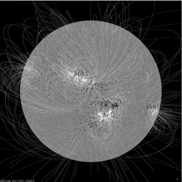
https://sdowww.lmsal.com/suntoday_v2/ n 1 Oct 2015bbHMI Blos with PFSS field lines
https://suntoday.lmsal.com/sdomedia/SunInTime/2017/10/01/f_HMImagpfss.jpg
https://solis.nso.edu/0/vsm/crmaps/8542l_cr2186-2205.html SOLIS Data
Peter MacNeice, NASA GSFC CCMC (CCMC Model Host)
https://ccmc.gsfc.nasa.gov/models/WSA~v.5.2/
https://suntoday.lmsal.com/sdomedia/SunInTime/2017/10/01/f_HMImagpfss.jpg
https://solis.nso.edu/0/vsm/crmaps/8542l_cr2186-2205.html SOLIS Data
Peter MacNeice, NASA GSFC CCMC (CCMC Model Host)
https://ccmc.gsfc.nasa.gov/models/WSA~v.5.2/
CITE THIS NOTEBOOK
CITE THIS NOTEBOOK
3D printing of solar coronal flux tubes: Wang-Sheeley-Arge model
by Gilmer Allen Gary
Wolfram Community, STAFF PICKS, November 27, 2024
https://community.wolfram.com/groups/-/m/t/3329673
by Gilmer Allen Gary
Wolfram Community, STAFF PICKS, November 27, 2024
https://community.wolfram.com/groups/-/m/t/3329673