This rigorous definition called “Epsilon Delta” is a first for the mathematician and is an excellent preview of how to speak and write the actual language. There are several mental pictures and statements of change that must be all included in one precision (mathematical) ”sentence” This is like looking in the side mirror, the “rear view mirror” and also paying attention to the road ahead (of course) . . . while driving on a freeway. And then turn to your passenger and say . . . “did you know this idiot coming up behind us on our left will pass us in 1.26795 seconds and plow into that dump truck ahead of us in 0.000166662 seconds less time than that”?
Wolfram Mathematica is also a standard word program (text), with multiple dropdown menus and pallets that will enable you to type in actual mathematics operators, symbols and arguments just as they appear in textbooks just for reading and not be calculated.
For those so inclined, unless you can do better, I believe the thing goes something like this . . .
∀ ϵ > 0 ∋ δ < 0 ∥ 0 ≺ [ x - a ] < δ ⇒ [ f (x) - L ] < ϵ
For Derivatives and Integrals, the simplest equation used to explore these concepts is This works because we can see the derivative is 2( and the indefinite integral is . But to tackle this definition and state it a s a proof with elegance we choose the next simple but more awkward numbers three and nine. But we will trap the nine in an argument that makes it go away ( (√ 9 - 3) = 0 ) and become a more “square” even looking function . . . to be arbitrated between two points.
2.
x
1
3
3
x
f[x_]:=N[
2x+1
-3]The N gives a Number . . . this will become the Limit 3 as X becomes 4
g[x_]:=
2x+1
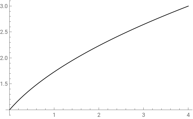
We begin the investigation without the limiting argument and just consider √2x+1
Plot[g[x],{x,0,4}]
Plot[-3+
1+2x
,{x,0,5}]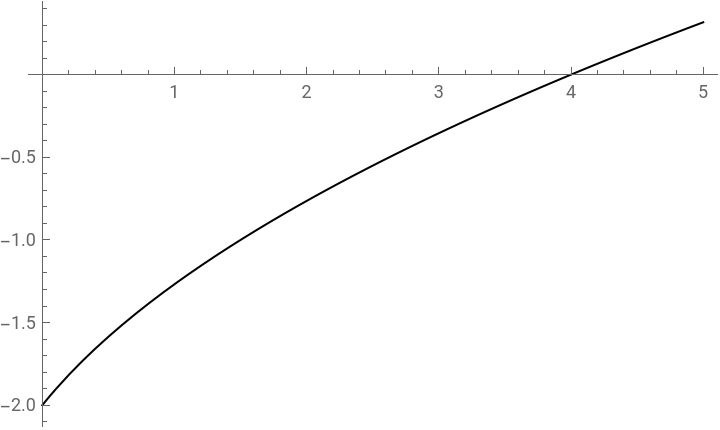
Above the plot shows the abscissa (x) has a maximum function value of 4
And below the plot shows that when the Limit is subtracted from this value as a Number the abscissa is where the argument is ZERO (the argument becomes the ordinate.)
And below the plot shows that when the Limit is subtracted from this value as a Number the abscissa is where the argument is ZERO (the argument becomes the ordinate.)
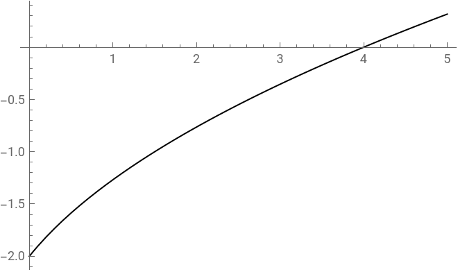
These two graphs above are NOT the same thing but the curve does appear similar in “shape”. There are no “nines” (9). But the magic number is 9 because the square root of that is three, which, when you subtract three . . . makes ZERO. The three and the four are showing up big in our investigation. Not 9, and when it does the whole thing become zero . . . IF AND ONLY IF . . .F(X) - L = ≻ 0 This makes the crucial argument that the absolute value is also something like the nine (9) and the square root function. Both of which have disappeared and we are now arbitrating between two physical distances from four and three. If you are a Lawyer, and you want to be a great Lawyer, learn how to state ,mathematical arguments, proofs and theorems, and thank the mathematician later.
9,(wichequalsthree)
2x+1
-3.
Plot[-3+
1+2x
,{x,3,5}]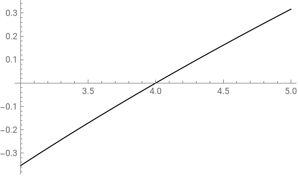
In the Wolfram Mathematica classroom / homework session, one is free to “call up” and “assign” just about anything that most describes whatever the mathematical understanding asks for . . .
Introducing . . . “distance from epsilon” . . . (this of course is a positive number (δ ≻ 0 ) from epsilon ϵ )
Introducing . . . “distance from epsilon” . . . (this of course is a positive number (δ ≻ 0 ) from epsilon ϵ )
distancefromepsilon={3.9,3.95,3.995,3.9995,4.0005,4.001,4.01,4.1}
{3.9,3.95,3.995,3.9995,4.0005,4.001,4.01,4.1}
ListLinePlot[distancefromepsilon]
Note carefuly where the two players 3 and four “appear” on this plot above. This time we are boxing in just the four ( the square root function). The three (3) only shows up when you look at and trace the line. As soon as three hits four the line seems to level until about seven point two “ish”, and then shoots up at the same slope it was approaching just before it hit three.
“did you know this idiot coming up behind us on our left will pass us in 4 seconds and plow into that dump truck ahead of us within 3 seconds less time than that”
“did you know this idiot coming up behind us on our left will pass us in 4 seconds and plow into that dump truck ahead of us within 3 seconds less time than that”
TableForm[distancefromepsilon]
3.9 |
3.95 |
3.995 |
3.9995 |
4.0005 |
4.001 |
4.01 |
4.1 |
f[4.0005]
0.000166662
f[1]
-1.26795
f[4]
0.
NumberForm[0.`,{20,19}]
0.0000000000000000000
f[3.9]
-0.0335206
f[5]
0.316625
Plot[g[x],{x,0,9}]
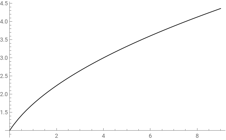
h={3.9,3.95,3.995,3.9995,4.0005,4.001,4.01,4.1}
{3.9,3.95,3.995,3.9995,4.0005,4.001,4.01,4.1}
secslope[a_,h_]:=(f[a+h]-f[a])/h
secline[a_,h_,x_]:=secslope[a,h](x-a)+f[a]
Manipulate[Plot[{f[x],secline[2,k,x]},{x,3,6},AspectRatio1,PlotRange{{0,8},{0,8}}],{k,3,.01}]

