This project explores reaction-diffusion dynamics using the Gray-Scott model and demonstrates how complex spatial patterns emerge from simple local rules on a discrete lattice. The simulation tracks the evolution of coupled chemical fields using a grid-based numerical implementation and monitors pattern development over long time scales. The analysis proceeds from model definition and numerical integration to visualization and statistical examination of the final patterns. The resulting structures are quantified using Fourier power spectra and spatial autocorrelation functions, which reveal a dominant wavelength, characteristic length scales, and long-range spatial coherence. These analyses show that the patterns possess stable, repeatable statistical structure determined by the model parameters rather than random noise. In the final section, the work briefly discusses how these measurable statistics provide a natural bridge to diffusion-based generative models, suggesting that reaction-diffusion systems can serve as structured training data for learning and reproducing physical pattern formation behavior.
Introduction: Reaction-Diffusion Systems
Introduction: Reaction-Diffusion Systems
The Gray-Scott model describes two chemical species u and v that diffuse and react according to the following partial differential equations: . In these equations, and are diffusion coefficients, is the feed rate, is the kill rate, and the term represents an autocatalytic reaction. Different combinations of and parameters produce spots, stripes, or chaotic patterns, forming what is known as a bifurcation atlas.
∂u ∂t D u 2 ∇ 2 v |
∂v ∂t D v 2 ∇ 2 v |
D
u
D
v
f
k
uv²
f
k
The implementation begins with defining the grid and time parameters. We use a grid size of 128 by 128 cells and simulate 20000 time steps. For the Gray-Scott parameters, we choose values optimized for spot-forming: = 0.16 for the diffusion coefficient, = 0.08 for the diffusion coefficient, = 0.030 for a feed rate, and = 0.055 for a kill rate. We also introduce an explicit time step = 0.25 to control the stability.
D
u
u
D
v
v
f
k
dt
ClearAll["Global`*"];gridSize = 128;timeSteps = 20000; Du = 0.16;Dv = 0.08;f = 0.030; k = 0.055; dt = 0.25;
We discretize the Laplacian operator using nearest-neighbor differences with periodic boundary conditions. The discrete approximation takes the form as followed: u≈+++-4. The time evolution uses an Euler forward scheme +ΔtF(,) with explicit time step scaling and value clamping. After computing the Laplacian of both fields and the reaction term , we update both concentration fields and clip the values to the range between 0 and 1.
2
∇
u
i+1,j
u
i-1,j
u
i,j+1
u
i,j-1
u
i,j
n+1
u
n
u
n
u
n
v
uvv
laplacian[m_] := RotateLeft[m, {1, 0}] + RotateRight[m, {1, 0}] + RotateLeft[m, {0, 1}] + RotateRight[m, {0, 1}] - 4 m;step[{u_, v_}] := Module[{Lu, Lv, uvv, uNew, vNew}, Lu = laplacian[u]; Lv = laplacian[v]; uvv = u v^2; uNew = u + dt * (Du Lu - uvv + f (1 - u)); vNew = v + dt * (Dv Lv + uvv - (f + k) v); uNew = Clip[uNew, {0.0, 1.0}]; vNew = Clip[vNew, {0.0, 1.0}]; {uNew, vNew}];
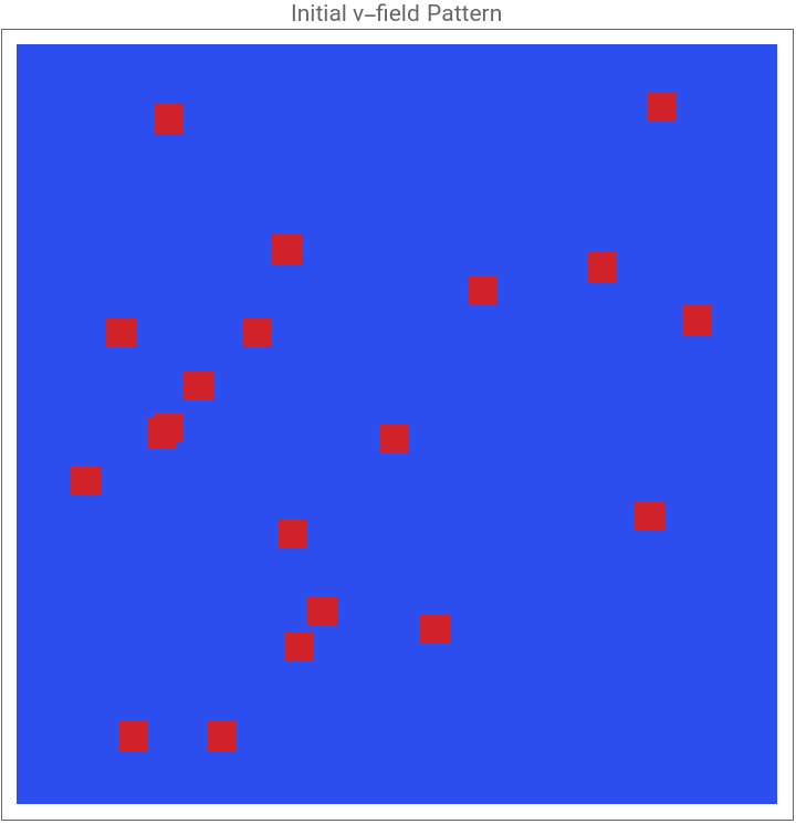
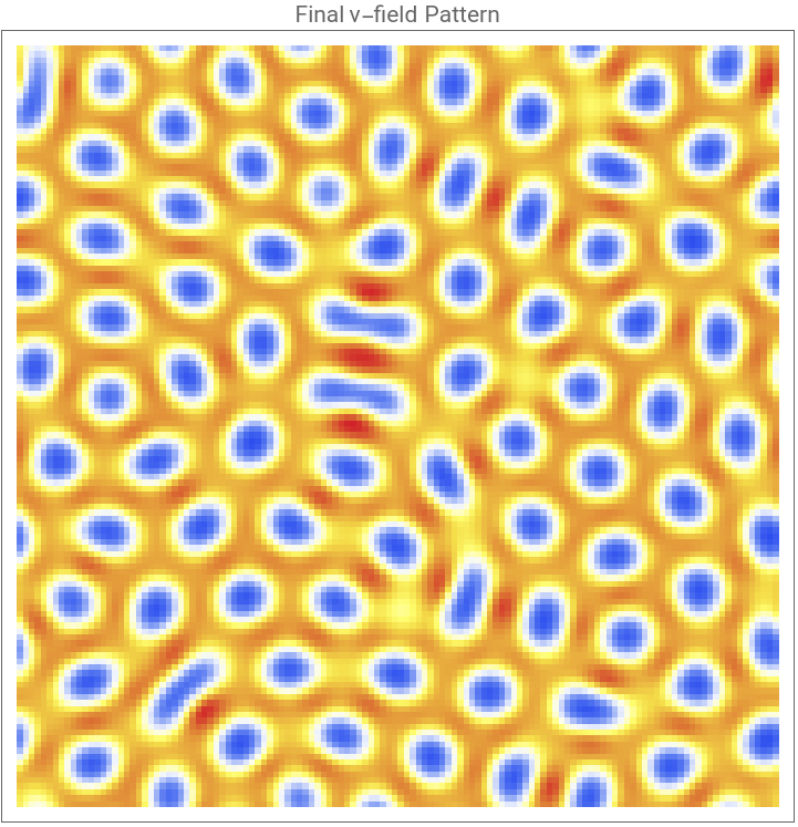
We initialize the system using an approach that works well for generating spot patterns. Instead of uniform random perturbations, we seed the domain with multiple localized spots at random positions. The u-field starts at 1.0 everywhere, while the v field starts at 0.0. We then add several circular seed regions where is reduced to 0.5 and is raised to 0.25. This seeding strategy provides strong initial perturbations that more reliably lead to well-formed spot patterns. We place 20 random seeds, each with a radius of approximately 3 grid units. The simulation proceeds by iteratively applying the update rules for 20000 time steps. This extended simulation time allows patterns to fully develop and stabilize. The evolution of the concentration field can be visualized through animation, showing snapshots at regular intervals of 80 time steps. The final pattern reveals the stable spatial structure that emerges from the initially seeded conditions. For the parameters chosen, the system develops a field of spots with characteristic spacing. We also examine basic statistics of the final field to verify that the pattern has developed properly, printing the range and standard deviation of the concentration values.
u
v
v
v
u = ConstantArray[1.0, {gridSize, gridSize}];v = ConstantArray[0.0, {gridSize, gridSize}];SeedRandom[456];numSeeds = 20;Do[ cx = RandomInteger[{10, gridSize - 10}]; cy = RandomInteger[{10, gridSize - 10}]; Do[ If[Norm[{i - cx, j - cy}] < 3, u[[i, j]] = 0.5; v[[i, j]] = 0.25; ], {i, cx - 3, cx + 3}, {j, cy - 3, cy + 3} ], {numSeeds}];
states = NestList[step, {u,v}, timeSteps];ListAnimate[ArrayPlot[#, ColorFunction->"TemperatureMap", ColorFunctionScaling->True, ImageSize->Medium, PlotLabel->"v concentration"] &/@states[[1;;-1;;80,2]], AnimationRate->40]ArrayPlot[v, ColorFunction->"TemperatureMap", ColorFunctionScaling->True, ImageSize->Medium, PlotLabel->"Initial v-field Pattern"]ArrayPlot[states[[-1,2]], ColorFunction->"TemperatureMap", PlotLabel->"Final v-field Pattern", ImageSize->Medium]vField = states[[-1,2]];Print["v field range: ", MinMax[vField]];Print["v field std dev: ", StandardDeviation[Flatten[vField]]];
Here is the link to the animation: https://drive.google.com/file/d/13IS3fApM_b-cH5GV9LR0nT4wQuED4f3l/view?usp=sharing
v field range: {0.0275997,0.301934}
v field std dev: 0.0691858
The evolution from initial to final v-field patterns demonstrates canonical Gray-Scott reaction-diffusion behavior. Beginning with sparse, randomly-distributed perturbations (20 localized red squares on a uniform blue background), the system undergoes spontaneous pattern formation through reaction and diffusion processes. The final steady-state pattern exhibits the expected Gray-Scott characteristics: self-replicating spot structures with distinct blue cores (low v-concentration) surrounded by white halos (intermediate v) embedded in a yellow-orange background matrix (high v). The v-field range of 0.028 to 0.302 with standard deviation 0.069 indicates moderate heterogeneity, reflecting the spatial organization into discrete chemical domains. The spot multiplication and space-filling behavior fulfill theoretical predictions for Gray-Scott systems, where initial perturbations start the formation of stable and localized structures that reproduce. The preservation of spot individuality even at high packing density confirms the system has reached a stable equilibrium pattern.
Spatial Structure Analysis
Spatial Structure Analysis
To quantify the spatial organization of the resulting pattern, we analyze its statistical properties through Fourier analysis. These statistical measures capture the essential features of the spot structure, including characteristic length scales and spatial periodicities. The Fourier transform reveals dominant spatial frequencies, which correspond to the characteristic wavelength of spots. We compute the power spectrum as the squared magnitude of the Fourier transform of the final v-field: where is the power spectrum, denotes the Fourier transform, is the v-field, and is the spatial mean. The spectrum is centered by shifting zero-frequency components to the center and displayed on a logarithmic scale to reveal the ring of power at the dominant wavenumber. The DC component (mean value) is removed by centering the v-field prior to the Fourier transform, enabling better visualization of the spatial frequencies that encode pattern structure. We examine the zoomed view of the central region to better observe the low-frequency components that correspond to the characteristic inter-spot spacing.
S(k)F[v(x)-〈v〉]
2
|
S(k)
F
v(x)
〈v〉
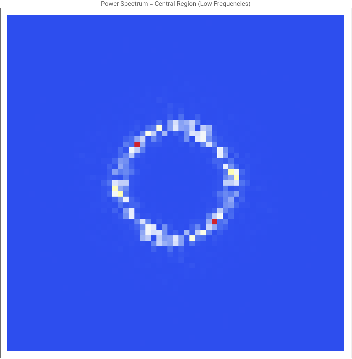
The Fourier power spectrum of the final v-field pattern shows the spatial periodicity and regularity of the emergent spot structures. The spectrum exhibits a prominent ring-shaped distribution of power concentrated at a specific radial frequency, indicating a well-defined characteristic wavelength dominating the spatial organization. This circular symmetry in frequency space corresponds to isotropic pattern formation, spots are evenly spaced in all directions with no preferred orientation, as expected for Gray-Scott systems on uniform lattices with isotropic diffusion. The ring’s radius directly encodes the typical inter-spot spacing distance, while the ring’s width indicates modest variation around this preferred scale. The presence of two distinct high-power peaks (visible as red spots at approximately opposing positions on the ring, upper-left and lower-right) suggests minor directional biases or artifacts from the discrete lattice geometry and periodic boundary conditions, but the overall circular structure confirms the pattern’s statistical isotropy. The concentration of power at low frequencies (central region of Fourier space) with minimal high-frequency content demonstrates that the pattern is dominated by smooth, regularly-spaced features. This spectral signature provides quantitative validation that the system has achieved a stable, periodic tiling pattern characteristic of Turing-type instabilities in the Gray-Scott model.
To quantify the dominant wavelength, we locate the maximum in the power spectrum and compute its distance from the center. This distance in Fourier space corresponds to the characteristic wavenumber, which can be converted to a real-space wavelength. The code prints the dominant wavelength in grid units and estimates how many structures fit across the domain.
Radially Averaged Power Spectrum
Radially Averaged Power Spectrum
Autocorrelation Function
Autocorrelation Function
Radial Autocorrelation
Radial Autocorrelation
Diffusion Models
Diffusion Models
Conclusion and Future Directions
Conclusion and Future Directions
We implemented the Gray–Scott reaction–diffusion system and observed spontaneous pattern formation from simple initial conditions. Power spectrum analysis revealed the dominant wavelength of the patterns, while autocorrelation measurements quantified coherence and characteristic length scales. These statistical tools showed that the patterns are not random, but follow stable, repeatable structures determined by the model parameters. Reaction–diffusion patterns also connect naturally to machine learning. A diffusion model trained on Gray–Scott data could generate new patterns without solving the PDE directly, as long as it reproduces key physical statistics such as dominant wavenumber, spot size distribution, and correlation length. Conditioning the model on the parameters f and k would allow it to generate patterns across different regimes and reflect the underlying bifurcation structure of the system. This approach highlights how physics-based simulations can provide structured training data and how statistical validation ensures that learned models capture real pattern-forming behavior rather than surface-level visuals.
References
References
◼
Gray, P., & Scott, S. K. (1984). Autocatalytic reactions in the isothermal, continuous stirred tank reactor: Oscillations and instabilities in the system A + 2B → 3B; B → C. Chemical Engineering Science, 39(6), 1087–1097. DOI: https://doi.org/10.1016/0009-2509(84)87017-7
◼
Pearson, J. E. (1993). Complex Patterns in a Simple System. Science, 261(5118), 189–192. DOI: https://doi.org/10.1126/science.261.5118.189
◼
Ho, J., Jain, A., & Abbeel, P. (2020). Denoising Diffusion Probabilistic Models. Advances in Neural Information Processing Systems, 33, 6840–6851. DOI: https://doi.org/10.48550/arXiv.2006.11239
◼
Song, Y., Sohl-Dickstein, J., Kingma, D. P., Kumar, A., Ermon, S., & Poole, B. (2021). Score-Based Generative Modeling through Stochastic Differential Equations International Conference on Learning Representations (ICLR). DOI: https://doi.org/10.48550/arXiv.2011.13456
◼
Here is the link to the full Wolfram Notebook: https://drive.google.com/file/d/1YauacbsgbsLQ_TXDDIWjZx1XmI-Idea2/view?usp=sharing
CITE THIS NOTEBOOK
CITE THIS NOTEBOOK
Reaction-diffusion on discrete lattices: pattern formation and spectral analysis
by Guhan Thiagarajan
Wolfram Community, STAFF PICKS, December 31, 2025
https://community.wolfram.com/groups/-/m/t/3599588
by Guhan Thiagarajan
Wolfram Community, STAFF PICKS, December 31, 2025
https://community.wolfram.com/groups/-/m/t/3599588