In this notebook, we extend Andrew Moylan’s technique for stabilizing the inverted circular pendulum in two dimensions via optimal control and the linear quadratic regulator (LQR) to the problem of stabilizing the inverted spherical pendulum in three dimensions. We end by speculating on machine-learning techniques for the LQR.
I have seen dozens of treatments of the circular pendulum. In fact, it’s often an undergraduate exercise in control theory. Inexplicably, I have found nothing useful on stabilizing the spherical pendulum. There is plenty of material on the swing-up problem and other non-linear regimes for the spherical pendulum, and those are much more complicated than stabilizing about the origin. However, a treatment of this stabilization problem, relevant in rocketry and robotics, is conspicuously difficult to find.
Moylan’s technique employs concise and beautiful symbolical derivation of the Euler-Lagrange equations as well as a satisfyingly simple linear quadratic regulator.
Background and Problem Statement
Background and Problem Statement
Andrew Moylan, formerly of Wolfram’s Technical Communication and Strategy group, wrote a blog in 2011 on stabilizing an inverted pendulum in two dimensions (https://blog.wolfram.com/2011/01/19/stabilized-inverted-pendulum/). The 2D pendulum moves in a circle about its base, and is thus called a circular pendulum. His approach is very attractive, and I follow it here.
Moylan promised a follow-on blog about stabilizing the inverted spherical pendulum in three dimensions, but I never found that blog. Here, we complete his blog series with the following scenario:
◼
Consider a massive thin rod, mounted to a spherical joint—the base—on a massless cart, free to slide without friction on a flat, level plane—the floor. “Thin” means ignoring the “spin” degree of freedom around the long axis of the rod (else we would have a Lagrange top). “Stabilizing” means self-centering at the origin of the generalized coordinate system with small generalized velocities, in the presence of perturbative forces applied at the base.
Moylan’s method has the following steps:
1
.Write full non-linear equations of motion in Euler-Lagrange form
2
.Linearize the equations about the unstable equilibrium point
3
.Compute the gain matrix of a Linear Quadratic Regulator
4
.Animate a trajectory of an instance of the problem
Non-Linear Equations of Motion
Non-Linear Equations of Motion
Global Constants
Global Constants
Acceleration of Earth’s gravitation; length of the pendulum as a thin rod; mass of the rod:
In[]:=
ClearAll[d,m,g];g=9.81;m=1;d=1;
Integration time:
In[]:=
ClearAll[tLim];tLim=30;(*seconds*)
Generalized Coordinates
Generalized Coordinates
The rod is anchored at its base in an idealized, frictionless, non-locking spherical joint free to slide on a level, flat plane. The generalized position coordinates of the base are and . The two angles of the standard spherical coordinate system describe the tilt of the rod: co-latitude θ—angle from vertical, and azimuth ϕ on the plane.
x
y
There are four degrees of freedom. The first-order state-space representation thus has eight variables: four generalized coordinates , , θ, ϕ, and four generalized velocities , yd, θd, ϕd, with the “d” denoting “overdot” or total time derivative.
x
y
xd
Potential energy
Potential energy
proportional to the height of the center of mass (CM) of the rod above the plane:
In[]:=
ClearAll[V];V[{x_,y_,θ_,ϕ_,xd_,yd_,θd_,ϕd_}]:=mgCos[θ];
d
2
Kinetic Energy
Kinetic Energy
There are two addends: kinetic energy of translation of the CM in the inertial , , frame and kinetic energy of rotation about the CM.
X
Y
Z
In[]:=
ClearAll[MI];MI=m;(*momentofinertiaofathinrod*)
1
12
2
d
To keep things easy, we’ll build up the velocities by hand, using Wolfram as an assistant.
Angular velocity measured in the inertial frame (by inspection):
In[]:=
ClearAll[ω];ω[{x_,y_,θ_,ϕ_,xd_,yd_,θd_,ϕd_}]:=+;
2
θd
2
ϕd
2
Sin[θ]
The CM of the rod in the inertial frame is at position
x[t]+ d 2 |
y[t]+ d 2 |
d 2 |
The following symbolical computation of derivatives ensures the inertial velocities of the CM:
In[]:=
With{drules={x[t]->x,y[t]->y,θ[t]->θ,ϕ[t]->ϕ,x'[t]->xd,y'[t]->yd,θ'[t]->θd,ϕ'[t]->ϕd}},Withvax=EchoDx[t]+Sin[θ[t]]Cos[ϕ[t]],t/.drules,vay=EchoDy[t]+Sin[θ[t]]Sin[ϕ[t]],t/.drules,vaz=EchoDCos[θ[t]],t/.drules,Null
d
2
d
2
d
2
»
xd+θdCos[θ]Cos[ϕ]-ϕdSin[θ]Sin[ϕ]
1
2
1
2
»
yd+ϕdCos[ϕ]Sin[θ]+θdCos[θ]Sin[ϕ]
1
2
1
2
»
-θdSin[θ]
1
2
Manually copy inertial velocities into the expression for kinetic energy (manual copying seems the most convenient way to get a function-like, Wolfram expression):
In[]:=
ClearAll[T];T[{x_,y_,θ_,ϕ_,xd_,yd_,θd_,ϕd_}]:=m+++MI(+);
1
2
2
xd+θdCos[θ]Cos[ϕ]-ϕdSin[θ]Sin[ϕ]
1
2
1
2
2
yd+ϕdCos[ϕ]Sin[θ]+θdCos[θ]Sin[ϕ]
1
2
1
2
2
-θdSin[θ]
1
2
1
2
2
θd
2
ϕd
2
Sin[θ]
Generalized Forces
Generalized Forces
The generalized, d’Alembertian forces that can work on virtual displacements δ and δ are just the actual forces [t],[t].
x
y
f
x
f
y
Generalized Torques
Generalized Torques
The torques of [t],[t] are applied at the point of contact, the spherical joint. Thus they do no virtual work applied to virtual displacements δθ and δϕ (I am not fully convinced of this point, but numerical simulation, the literature, and the visibly plausible results here support it).
f
x
f
y
Euler-Lagrange Equations
Euler-Lagrange Equations
The Euler-Lagrange equations follow via Wolfram symbolics, letting the coordinates and velocities vary independently of one another. Leqns are the Euler-Lagrange equations straight up. Seqns are the equations solved for the second-order terms and sorted into , , θ, ϕ order. The results are uninstructive, but displayed here for completeness.
x
y
In[]:=
ClearAll[L,x,y,θ,ϕ,fx,fy,Leqns,Seqns];L[{x_,y_,θ_,ϕ_,xd_,yd_,θd_,ϕd_}]:=T[{x,y,θ,ϕ,xd,yd,θd,ϕd}]-V[{x,y,θ,ϕ,xd,yd,θd,ϕd}];With[{Lcrds={x[t],y[t],θ[t],ϕ[t]}},With[{Lvels=D[Lcrds,t]},With[{Lncnf={fx[t],fy[t],0,0}},Leqns=Flatten@MapThread[{q,v,f}D[D[L[Lcrds~Join~Lvels],v],t]-D[L[Lcrds~Join~Lvels],q]==f,{Lcrds,Lvels,Lncnf}]]]];(Seqns=((Solve[Leqns,{x''[t],y''[t],θ''[t],ϕ''[t]}]//FullSimplify)[[1]]/.{Rule->Equal}))//TableForm
Out[]//TableForm=
′′ x (1.-1.2326× -32 10 -32 10 -32 10 2 Sin[θ[t]] 2 ′ θ -16 10 3 Sin[θ[t]] 2 ′ ϕ 0.333333+1. 2 Sin[θ[t]] |
′′ y (2.19444-2.Cos[2θ[t]]+0.25Cos[4θ[t]]+(1.08333-1.33333Cos[2θ[t]]+0.25Cos[4θ[t]])Cos[2ϕ[t]])fy[t]+(-1.08333+1.33333Cos[2θ[t]]-0.25Cos[4θ[t]])fx[t]Sin[2ϕ[t]]+Sin[ϕ[t]](-4.0875Sin[2θ[t]]+1.22625Sin[4θ[t]]+(0.722222Sin[θ[t]]-0.166667Sin[3θ[t]]) 2 ′ θ 2 ′ ϕ 2 (0.333333+1. 2 Sin[θ[t]] |
′′ θ 21.255Sin[θ[t]]-4.905Sin[3θ[t]]+Cos[θ[t]](-0.666667-2. 2 Sin[θ[t]] 2 ′ θ 2 ′ ϕ 2 (0.333333+1. 2 Sin[θ[t]] |
′′ ϕ Cos[ϕ[t]]Csc[θ[t]](-54.-36. 2 Csc[θ[t]] 4 Csc[θ[t]] 2 Csc[θ[t]] 4 Csc[θ[t]] 2 (3.+1. 2 Csc[θ[t]] ′ θ ′ ϕ 2 (3.+1. 2 Csc[θ[t]] |
Numerical Verification of Free Motion
Numerical Verification of Free Motion
Drop the pendulum from not-quite-upright and just off the X-axis. If the initial angles are too small, the numerical solution will have inadequate conservation of energy and not act plausibly. However, Wolfram’s numerical integrators have no other difficulty with these substantially non-linear equations. That, itself, is remarkable.
In[]:=
ClearAll[initialCoLatitudeRad,initialAzimuthRad];initialCoLatitudeRad=0.01;(*don'tmakemuchsmallerthanthis*)initialAzimuthRad=0.01;
In[]:=
ClearAll[ndsoln];ndsoln=NDSolve[Join[Seqns/.{fx[t]0,fy[t]->0},{x[0]x'[0]θ'[0]0,θ[0]
initialCoLatitudeRad
},{y[0]==y'[0]==0,ϕ'[0]==0,ϕ[0]==initialAzimuthRad
}],{x,y,θ,ϕ},{t,0,tLim}]Out[]=
xInterpolatingFunction,yInterpolatingFunction,θInterpolatingFunction,ϕInterpolatingFunction


In[]:=
Plot[{ndsoln[[1,1,2]][t],ndsoln[[1,2,2]][t],ndsoln[[1,3,2]][t]/(2π)},{t,1,10},PlotLegends->{"x","y","θ"},Frame->True,FrameLabel->{"time [s]","meters or radians"}]
Out[]=
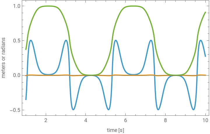


The following animation of free motion produces plausible back and forth swinging, verifying the non-linear equations of motion. The same simulation and animation routines work when we apply forces later.
Linearized Equations of Motion
Linearized Equations of Motion
State-Space Model
State-Space Model
by inspection of the linearized equations:
Trust, but Verify
Trust, but Verify
Wolfram' s StateSpaceModel also directly renders the reduced equations about the origin into standard state-space form, exactly as above:
LQR Gains
LQR Gains
These matrices are tuned by the controls engineer to meet given requirements. In our case, identity matrices suffice for a plausible result, and that’s all we’re trying to achieve here.
Control Force
Control Force
The grand beauty of this scheme is that the two forces we need to apply to the base are simply this 2x6 matrix times the 6D state residual or state error, that is, the difference between the current state and the desired configurations and velocities. In our case, since the desired configurations and velocities are zero, we just multiply the gains times the state.
WARNING: the LQR only works when the residuals are small, that is, when the linear approximations of the equations of motion are good enough. We shall see that this regime is larger than might be first thought. The great complexities of the control problem for the spherical pendulum arise in the non-linear regimes when the residuals are large, but we don’t consider those regimes in this notebook. However, we shall see that you can really kick the system hard and still recover.
First, check that the system stabilizes when there are no disturbances.
Now, come up with some hard bumps (a-la Moylan) for the first 15 seconds and watch the system recover in the last 15 seconds. This is really cool!
Machine Learning for the LQR
Machine Learning for the LQR
In earlier work, I wrote about human-preference learning for the gains matrix, directly, by humans iteratively choosing between pairs of randomly generated gains matrices within ever-decreasing bounds until converging on an acceptable one. That scheme requires learning DOF x force-dim parameters, the dimensions of the gains matrix. That is small in this case, but consider a real robot with hundreds or thousands of degrees of freedom and dozens or hundreds of force actuators and see that the problem is explosive.
CITE THIS NOTEBOOK
CITE THIS NOTEBOOK
Stabilizing the spherical pendulum from scratch
by Brian Beckman
Wolfram Community, STAFF PICKS, November 19, 2025
https://community.wolfram.com/groups/-/m/t/3577845
by Brian Beckman
Wolfram Community, STAFF PICKS, November 19, 2025
https://community.wolfram.com/groups/-/m/t/3577845