Introduction
Introduction
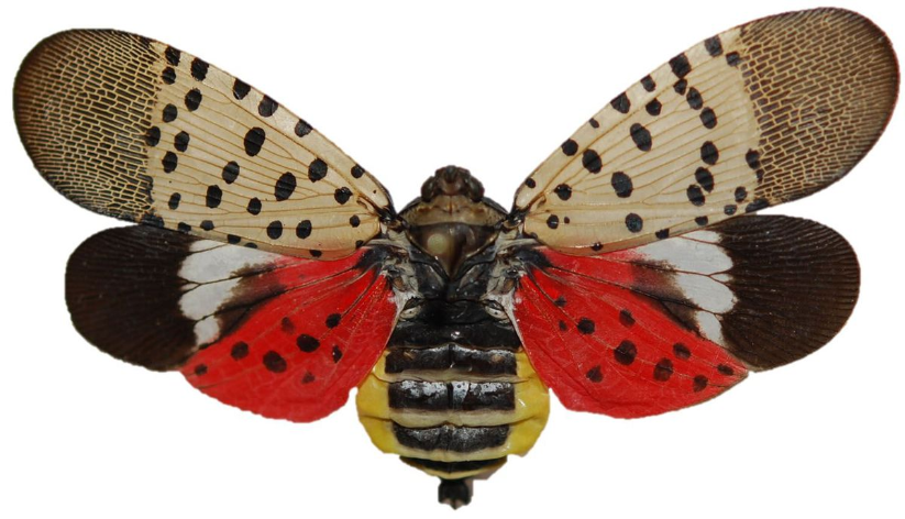
For my Honors Project at school, I worked on this project concerning the spotted lanternfly (SLF) (Lycorma delicatula), an invasive species. With the rise of globalization, there has been a critical threat to wildlife spreading throughout the world--invasive species. Invasive species are living organisms that come from a foreign country that out-compete or infect local wildlife. The negative impact is seen far and wide from agriculture to biodiversity to the global economy. This project is particularly concerned about the geographical spread of an invasive species after establishment in a different location.
Originally native to China, India, and Vietnam, it was first spotted in Berks County, Pennsylvania in September 2014. The SLF has attacked many hardwood trees and fruits, especially grape crops, and this poses a significant threat to the 18 billion dollar Pennsylvania agricultural industries.
Originally native to China, India, and Vietnam, it was first spotted in Berks County, Pennsylvania in September 2014. The SLF has attacked many hardwood trees and fruits, especially grape crops, and this poses a significant threat to the 18 billion dollar Pennsylvania agricultural industries.
Model
Model
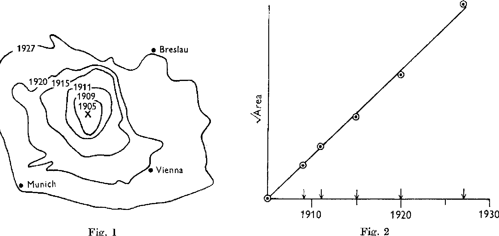
The goal is to be able to accurately predict the geographic spread of the Spotted Lanternfly using a mathematical model. With proper predictions of dispersal, preventative measures and management strategies may be implemented and other studies and actions can be conducted to minimize the impact.In 1953, J. G. Skellam wrote the paper “Random Dispersal in Theoretical Populations that presents a theory about the spread of an invasive species. Partial differential equations have been used to model the spread of many invasive species, such as the muskrat (Ondatra zibethicus L.) in Europe and gypsy moth (Lymantria dispar) in America. Muskrats, semi-aquatic rodents, were first introduced near Prague in 1909. The areas that muskrats inhabited at different time points were calculated. Assuming a circular spread pattern, Skellam took the square root of each area and plotted them against the time of measurement , where the area enclosed by a theoretical contour is regarded as an estimate of pi r^2 and the square root of it represents the theoretical radius of the expanding circle. It was found that there was a very strong linear correlation between the two. I used a similar model and available data to estimate spreading parameters.
Pennsylvania Department of Agriculture Data
Pennsylvania Department of Agriculture Data
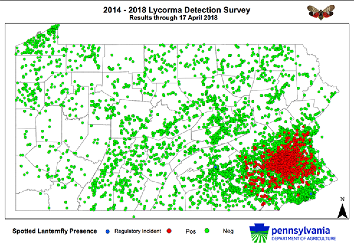
Historical SLF distribution data was collected from the Pennsylvania Department of Agriculture (PADA) website. The red indicates positive SLF occurrence, while the green or blue represents negative occurrence or a regulatory incident. Although the SLF has also been reported in other states, it is probable that they moved to these places through motor vehicles not natural dispersal, so only data from southeast PA was used. This data was collected from October 2015-December 2018.
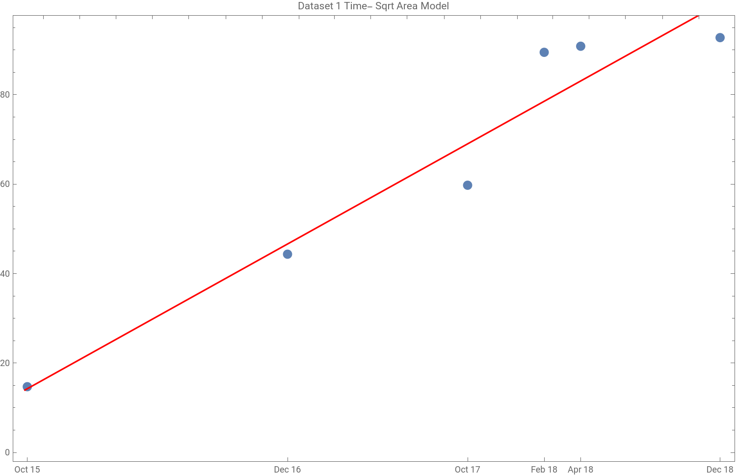
I used multiple trials of Sketch and Calc irregular area calculator measurements to find the approximate area of infestation at each time. Since we are assuming that the spread is in a circular pattern, we will square root each of the areas before generating the linear model. Here, we define the dataset, create the TimeSeries, and make a plot of the data points and line.
Define the times for Dataset 1
In[]:=
times1={"October 5, 2015","December 13, 2016","October 10, 2017","February 15, 2018","April 17, 2018","December 6, 2018"};
Define the areas for Dataset 1
In[]:=
areas1={216.235,1964.995,3569.9125,8004.2475,8249.505,8603.245};
Square root the areas
In[]:=
sqrtareas1=Map[Sqrt[#]&,areas1]
Out[]=
{14.7049,44.3283,59.7487,89.4665,90.8268,92.7537}
Create the time series
In[]:=
data1=TimeSeries[Transpose[{times1,sqrtareas1}]]
Out[]=
TimeSeries


Plot the points
In[]:=
plotdata1=DateListPlot[data1,JoinedFalse,DateTicksFormat->{"MonthNameShort"," ","YearShort"},FrameTicks{{Automatic,Automatic},{times1,Automatic}},ImageSize750,PlotLabel"Dataset 1 Time- Sqrt Area Model"];
Find linear model and plot it
In[]:=
equation1=LinearModelFit[data1,x,x];linedata1=Plot[Normal@equation1,{x,AbsoluteTime["October 2015"],AbsoluteTime["December 2018"]},PlotStyleRed,ImageSize750,AxesLabel{"Time","Area (km^2)"}];
This is the resulting equation and plot
In[]:=
Normal@equation1
Out[]=
-3130.75+8.60939×x
-7
10
Show both plots
In[]:=
plotline1=Show[plotdata1,linedata1]
Out[]=
In order to calculate the rate of spread per year, we must multiply by the number of seconds per year and divide by the square root of pi.
In[]:=
peryear[x_]:=Quantity[Last@x["BestFitParameters"],"km/s"]*UnitConvert,"Seconds"Quantity[Sqrt[Pi],"year"]
In[]:=
rate1=peryear[equation1]
Out[]=
Find and graph the residual
Find R-squared value
I created the following functions to do all of the above steps and display the final results with any input of times and areas.
Model 1
Model 1
In this model, the rate of spread per year would be 15.318 km/yr, meaning the radius of the area of infestation would increase by 15.345 km/yr. I then decided to remove the 4th and 5th data points, since they may have skewed the line upwards and were collected from a different season than the other four points.
Model 2
Model 2
This model is more linear, with a R-Squared value of 0.995, and the rate of spread is now 13.665 km/yr.
New York State Integrated Pest Management Data
New York State Integrated Pest Management Data
After December 2018, specific survey-point data was no longer available to the public. Maps were released by the New York State Integrated Pest Management Program, that showed counties that contained SLF infestation and reported sightings. The blue areas represent infestation areas, red lines represent quarantine boundaries, and yellow represents SLF found, but no infestation. Only the infestation were considered in calculating the spread rate because it is assumed that isolated incidents is due to human activity and not natural dispersion.
I observed and identified which counties were infested with the SLF for each time measurement and created the dataset below.
Create the dataset
To more clearly visualize the geographic area, I created this animation of maps.
Next, I needed to calculate the total area of infestation at each time. I also needed to delete all the cases in Virginia because I assumed that they were not due to natural spread.
Delete cases in Virginia
Calculate the total area for each time
Create the times list
After this, I could run the data and create the model as like before.
Model 3
Model 3
Generate the model
I think this dataset was not as accurate in predicting spread likely due to the fact that it was collected over the time period of a year rather than 3 years, and it used complete counties rather than specific geographic points. This means that a singular infestation in part of a county would count as the entire county, so the rate is likely overstated.
Both Datasets Combined
Both Datasets Combined
Lastly, I combined both datasets and created a model from that. I had to first make them the same format, by using the first datasets’ maps and identifying the entire counties of infestation, which will make the data more consistent. I also created another map animation.
Create new data from Dataset 1 and map it
Combine the datasets and create the model
Model 4
Model 4
This model is actually the second most linear with a R-Squared value of 0.980 and a rate of spread of 18.1746 km/yr.
Conclusion
Conclusion
With different data, we are able to make several approximate predictions for the rate of spatial spread of Lycorma Delicatula in the United States. The most accurate rate is likely the 13.665 km/yr from the model with the greatest R-Squared value. This is because it used geographic point data rather than the county data and were collected at approximately the same season (October-December), accounting for seasonal differences in SLF reproduction. In the following simulation, you can visualize how far the SLF is predicted to reach using the 4 calculated rates of spread, where n is the years from initial SLF introduction in Berks County, PA and k is the rate of spread.
The theoretical prediction given here can be tested and validated through future SLF survey data. While our data fits with the diffusion equation extremely well, it was calculated for only a small area in southeast Pennsylvania, which is geographically quite homogeneous. It is known that spatial heterogeneity, availability of SLF host plants, and climate can affect the invasion speed. Furthermore, local governments have implemented a quarantine in several counties and other eradication methods. This definitely has an effect on the diffusion of the insect. In the future, the model can be improved by incorporating these factors.
In the future, I hope to play around with only using the data from certain seasons and use any future data to improve the accuracy of the model.
References
References
[1] Pennsylvania Department of Agriculture.
[2] L.Barringer, L.Donovall, S.Spichiger, D.Lynch, and D.Henry.The first new world record of lycorma delicatula.Entomological news, 125 (1) : 20–23, 2015.
[3] E.Dobbs.Sketch and Calc, Feb 2011.
[4] J.Jung, S.Jung, D.Byeon, and W.Lee.Model - based prediction of potential distribution of the invasive insect pest, spotted lanternfly lycorma delicatula, by using climex.Journal of Asia - Pacific Biodiversity, 10 (4) : 532–538, 2017.
[5] Elaine Lidholm. Frederick county.
[6] J. L. Lockwood, M. F. Hoopes, and M. P. Marchetti. Invasion ecology. John Wiley & Sons, 2013.
[7] J. Skellam. Random dispersal in theoretical populations. Biometrika, 38(1/2):196–218, 1951.
[8] Tewodros T Wakie, Lisa G Neven, Wee L Yee, and Zhaozhi Lu. The establishment risk of lycorma delicatula (hemiptera: Fulgoridae) in the united states and
globally. Journal of Economic Entomology , 2019