Quasilinear Solution Sequence for Nonlinear Tubular Reactor with Dispersion
Authors: Housam Binous and Ahmed Bellagi
Quasilinear Solution Sequence for Nonlinear Tubular Reactor with Dispersion
Authors: Housam Binous and Ahmed Bellagi
Authors: Housam Binous and Ahmed Bellagi
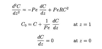
Consider a second-order chemical reaction 2A → B occurring in a tubular reactor with axial dispersion .
The governing equation can be found in Ref. 1.
The boundary conditions are the Danckwerts boundary conditions, which make the problem a split boundary condition problem.
We solve this problem with NDSolve and with orthogonal collocation.
Description of the orthogonal collocation method using Chebyshev-Gauss-Lobatto points is given in the following paper:
H. Binous, A. Shaikh and A. Bellagi, Chebyshev Orthogonal Collocation Technique to Solve Transport Phenomena Problems With Matlab and Mathematica, Computer Applications in Engineering Education, 23(3), pp. 422–431, 2015.
Linearizing the ODE about an assumed solution and performing a sequence of four iterations gives the same solution to this problem as NDSolve and orthogonal collocation.
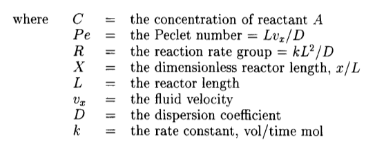
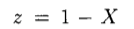
Governing equations can be found in Ref. 1: taking place in a tubular reactor in which there is axial mixing.and .Reference:1- W. F. Ramirez, Computational Methods for Process Simulation, 2nd Edition, Oxford: Butterworth Heinemann, 1997, pp. 327-330.
In[]:=
Off[NDSolve::"bvluc"]
Solution of a split boundary problem with nonlinear term using NDSolve.
In[]:=
Pe=10;R=0.5;C0=5;
In[]:=
SOL=NDSolve[{D[c[z],{z,2}]-PeD[c[z],{z,1}]+PeRc[z]^2,C0c[1]+1/Pe(D[c[z],{z,1}]/.z1),(D[c[z],{z,1}]0/.z0)},{c[z]},{z,0,1}]
Out[]=
c[z]InterpolatingFunction[z]


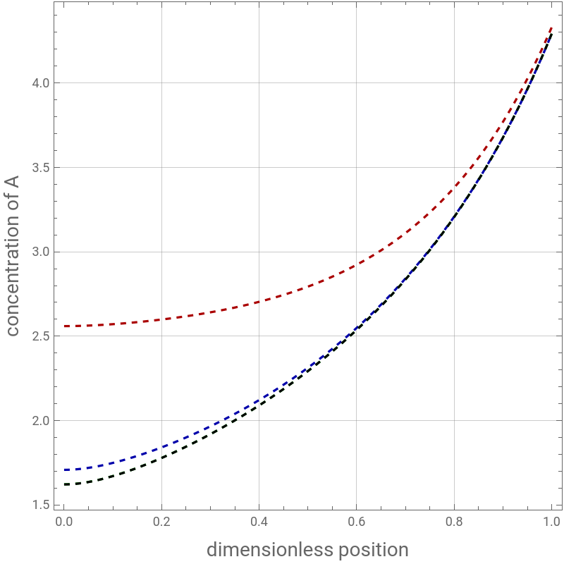
We assume a starting solution as constant concentration = 5. We then proceed with the quasilinear sequence until we get convergence to the solution of the original problem. Here four iterations are sufficient.

In[]:=
C0=5;
In[]:=
sol1=NDSolve[{D[c[z],{z,2}]-PeD[c[z],{z,1}]+2PeRc[z]C0-PeRC0^2,C0c[1]+1/Pec'[1],(D[c[z],{z,1}]0/.z0)},{c[z]},{z,0,1}]
Out[]=
c[z]InterpolatingFunction[z]

In[]:=
C0=First[c[z]/.sol1]
Out[]=
InterpolatingFunction[z]
In[]:=
sol2=NDSolve[{D[c[z],{z,2}]-PeD[c[z],{z,1}]+2PeRc[z]C0-PeRC0^2,5c[1]+1/Pec'[1],(D[c[z],{z,1}]0/.z0)},{c[z]},{z,0,1}]
Out[]=
c[z]InterpolatingFunction[z]

In[]:=
C0=First[c[z]/.sol2]
Out[]=
InterpolatingFunction[z]
In[]:=
sol3=NDSolve[{D[c[z],{z,2}]-PeD[c[z],{z,1}]+2PeRc[z]C0-PeRC0^2,5c[1]+1/Pec'[1],(D[c[z],{z,1}]0/.z0)},{c[z]},{z,0,1}]
Out[]=
c[z]InterpolatingFunction[z]

In[]:=
C0=First[c[z]/.sol3]
Out[]=
InterpolatingFunction[z]
In[]:=
sol4=NDSolve[{D[c[z],{z,2}]-PeD[c[z],{z,1}]+2PeRc[z]C0-PeRC0^2,5c[1]+1/Pec'[1],(D[c[z],{z,1}]0/.z0)},{c[z]},{z,0,1}]
Out[]=
c[z]InterpolatingFunction[z]

Results for the four iterations are plotted on the same graph below.
The 3rd and 4th iterations coincide indicating convergence .
The 3rd and 4th iterations coincide indicating convergence .
In[]:=
Plot[{c[z]/.sol1,c[z]/.sol2,c[z]/.sol3,c[z]/.sol4},{z,0,1},PlotRangeAll,PlotStyle{{Darker@Red,Dashed},{Darker@Blue,Dashed},{Darker@Green,Dashed},{Black,Dashed}},Frame->True,GridLines->Automatic,FrameLabel->{Style["dimensionless position",14],Style["concentration of A",14]},ImageSize->400{1,1},AspectRatio->1,PlotLegends->{Style["1st iteration",14,Darker@Red],Style["2nd iteration",14,Darker@Blue],Style["3rd iteration",14,Darker@Green],Style["4th iteration",14,Black]}]
Out[]=


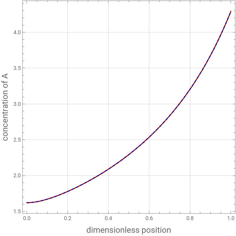
Results obtained with NDSolve and the iterative technique are identical.
In[]:=
Plot[{c[z]/.sol4,c[z]/.SOL},{z,0,1},PlotStyle{{Darker@Red},{Darker@Blue,Dashed}},Frame->True,GridLines->Automatic,FrameLabel->{Style["dimensionless position",14],Style["concentration of A",14]},ImageSize->400{1,1},AspectRatio->1,PlotLegends->{Style["4th iteration",14,Darker@Red],Style["NDSolve",14,Darker@Blue]}]
Out[]=

Solution using orthogonal Collocation and Chebyshev-Gauss-Lobatto points
Comparison results with NDSolve (solid red line) and orthogonal collocation solution (gray dots)