Introduction
In 1901 the brilliant mathematician David Hilbert at Sorbonne posed the following question: can we construct an automated procedure to find/prove all the theorems of a mathematical theory? e. g. Arithmetic, Calculus, Set Theory, etc. Hilbert believed that such a procedure could be found. To Hilbert’s surprise, Kurt Gödel and Alan Turing proved that it was not possible. The amazing way in which Alan Turing found the proof that such a procedure was not possible brought the new era of digital computing and the birth of computer science.
Alan Turing created a machine, which now bears his name, to prove the impossibility of what Hilbert was proposing. The Turing Machine, (TM), is an automaton with 5-tuples (5 distinguishable elements) of which a Tape (memory), a Head that can read/write and a set of States (operations) stand out. The Turing Machine is deterministic automaton and its power rested with the Tape.
However, one might think that using the Turing Machine we can know when a problem is computable, that is, if the TM that can solve this problem. The reality is that we cannot know it since we cannot know for sure if a TM will reach the Halt state and stop. This is known as the Halting problem.
The Halting Problem is the Principle of indeterminacy of computer science; you can’t tell when an automated procedure is going to halt. The Busy Beaver, (BB), problem uses the TM as an automated procedure and is said to be an uncomputable problem for the aforementioned reason. The BB consists of finding the TM of a given size that takes the longest computational time to halt.
In this project we will use an unconventional Cellular Automaton (CA) as an automated procedure. That is, a 2-state CA with non-adjacent parent cells and estimate the Computational Universe by finding both the rules and the effects of initial conditions that lead to the Busy Beaver for these CAs. The CA model is equivalent to the TM model. The results of this project can be of great help since there is a conjecture that proposes that BB as candidates to be Turing Universality.
What is novel about it?
What is novel about it?
◼
The Busy Beaver for a CAs is not define.
◼
It’s clear for a TM.
◼
For a CA
A particular Initial Condition
A particular Code Rule
The Halt State is the x-space with all cells white (0´s)
The Busy Beaver is the CA Rule Code that takes the longest t-step to find the Halt State.
◼
Unconventional CAs
◼
A CAs with non-adjacent parent cells
What?
What?
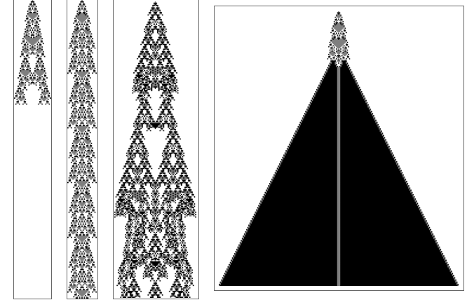
The figures shown below were taken from the page 69 of the book A New Kind of Science by Stephen Wolfram. The figure shows a totalistic three colors cellular automaton. A totalistic cellular automata, (TCA), in which the rules depend on the average of the values of the cells in a neighborhood. The left TCA reach the halt state, while the others never do or so it seems. What determines this behavior? Does it depend on the code rule? The initial condition? about what?
In[]:=
Grid[{{ArrayPlot[CellularAutomaton[{357,{3,1}},{{1},0},250]],ArrayPlot[CellularAutomaton[{600,{3,1}},{{1},0},250]],ArrayPlot[CellularAutomaton[{1599,{3,1}},{{1},0},250]],ArrayPlot[CellularAutomaton[{2058,{3,1}},{{1},0},250]]}}]
General and Particular Goals
General and Particular Goals
To answer the questions in the previous paragraph, the project will have the following goals .
◼
General
◼
To identify the Busy Beaver for an specific CA
◼
To measure algorithmic information content and complexity
◼
Particular
◼
To Determine the appropriate range r for the CAs
◼
The range r goes form 1,2,3, up to 4
◼
To determine the appropriate gaps for those Unconventional CAs
◼
Gaps = To skip first, second, third, etc. neighbour
◼
The Gaps will increase the multiplicity
◼
To determine a specific initial condition pattern
◼
To determine a particular neighbor patterns (range plus gaps) to study
Particular
Particular
For the regular TCA, without gaps, we have the following states and rules :
The appropriate range r
The appropriate range r
Out[]=
Neighbors | 1 | 2 | 3 | 4 | 5 | 6 | 7 |
Number of States | 2 | 3 | 4 | 5 | 6 | 7 | 8 |
Number of TCAs | 4 | 8 | 16 | 32 | 64 | 128 | 256 |
What is an Unconventional TCA and the Preliminary Tests
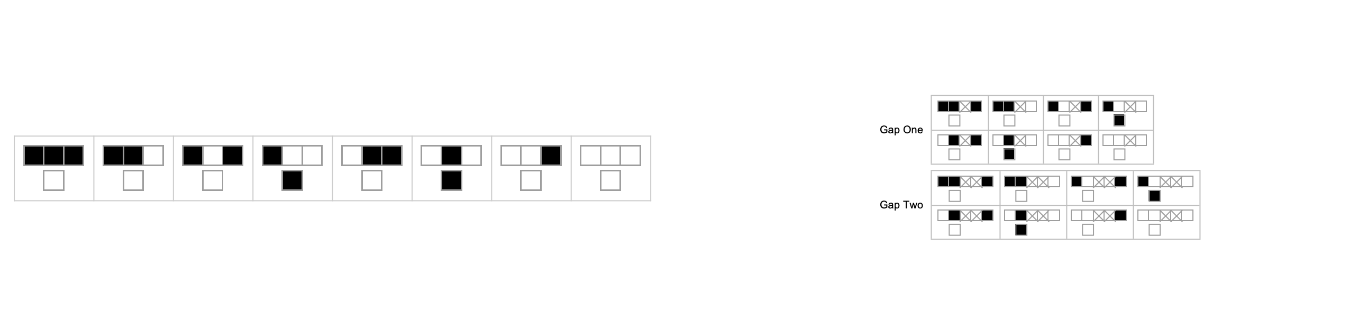
The Code Rules that govern the regular TCAs are affected by gapping between neighboring cells . In the next part we will take an example to clarify the concept of TCA.
TCA Code Rule 20, k-2 , r-1 ,
TCA Code Rule 20, k-2 , r-1 ,
In[]:=
GraphicsGrid[{{RulePlot[CellularAutomaton[{20,2,1}]],Grid[{{"Gap One",rulePlot[CellularAutomaton[{20,2,{{-1},{0},{2}}}]]},{"Gap Two",rulePlot[CellularAutomaton[{20,2,{{-1},{0},{3}}}]]}},AlignmentLeft]}},ImageSizeFull]
Out[]=
Is that all?
Is that all?
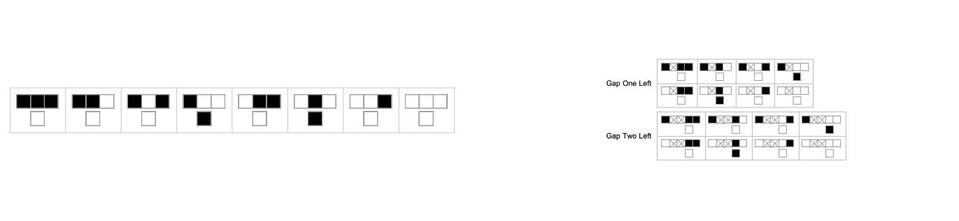
The skipping can be to the left of the center cell too
In[]:=
GraphicsGrid[{{RulePlot[CellularAutomaton[{20,2,1}]],Grid[{{"Gap One Left",rulePlot[CellularAutomaton[{20,2,{{-2},{0},{1}}}]]},{"Gap Two Left",rulePlot[CellularAutomaton[{20,2,{{-3},{0},{1}}}]]}},AlignmentLeft]}},ImageSizeFull]
Out[]=
Is it really all?
Is it really all?
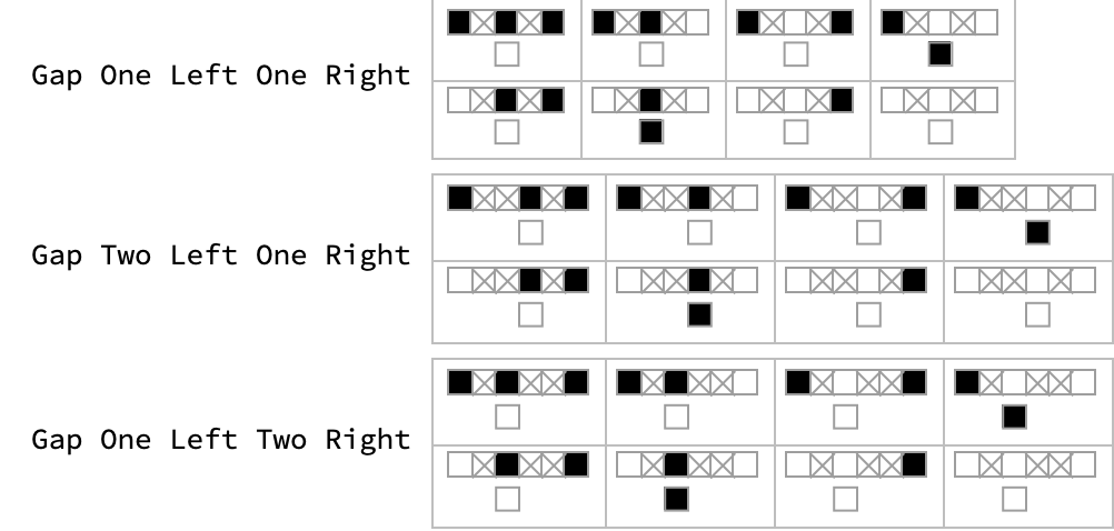
No! The skipping can be to the left and to the right of the center cell
In[]:=
Grid[{{"Gap One Left One Right",rulePlot[CellularAutomaton[{20,2,{{-2},{0},{2}}}]]},{"Gap Two Left One Right",rulePlot[CellularAutomaton[{20,2,{{-3},{0},{2}}}]]},{"Gap One Left Two Right",rulePlot[CellularAutomaton[{20,2,{{-2},{0},{3}}}]]}},AlignmentLeft]
The Zero Test
The Zero Test
Computational Universe of a TCA of 2-k, r-2
Computational Universe of a TCA of 2-k, r-2
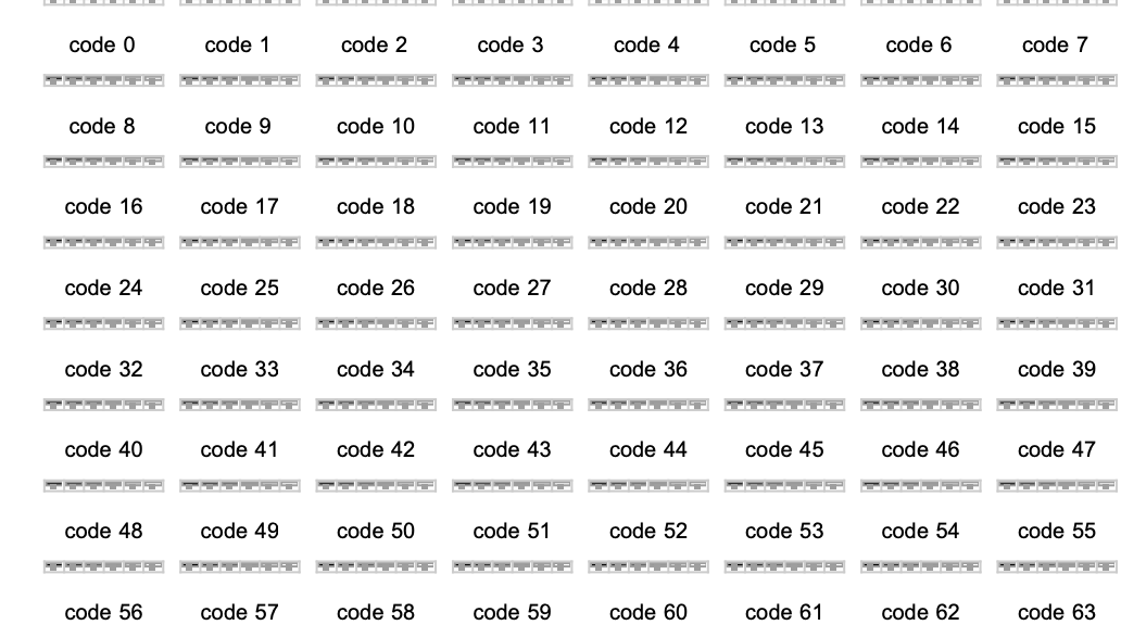
For this case there are 64 rules, so I' m able to map all of them . It' s important to mention that de Busy Beaver will depend on both, the code rule and the initial condition . Thai is, a different code rule or a different initial condition will give different Busy Beaver .
In[]:=
GraphicsGrid[Partition[Table[RulePlot[CellularAutomaton[{i,{2,1},2}],PlotLegends"Text"],{i,0,63}],8],ImageSize{785,469},AspectRatioFull]
The Code Rule 20
In[]:=
RulePlot[CellularAutomaton[{20,{2,1},2}],PlotLegends"Text"]
Initial Condition
Initial Condition
Out[]=
| ||||
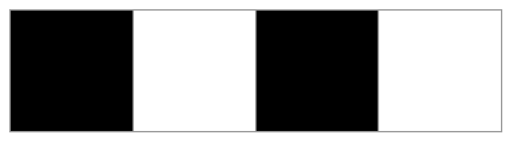
In[]:=
tca20=CellularAutomaton[{20,{2,1},2},{{1,0,1},0},{10,{-15,15}}];ArrayPlot@tca20
Out[]=
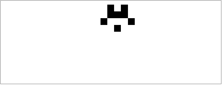
The following image shows the evolution of the TCAs according to the width considered. That is, we vary the width to see the dynamics of the BBs that appear with it and compared with the All the option at the end.
The following image shows the history of each of the TCA rule that reached the Halt state a
The Complexity Measure
The Complexity Measure
The measurement of complexity has always been a real challenge in the world of science . Knowing how random an object is, being the object a way of abstracting a part of the universe - a system -, has given rise to great revolutions . For example, the revolution of matter that allowed human beings to be sedentary and form societies, develop agriculture and livestock . The industrial revolution with the avenue of Thermodynamics and the informatics revolution that we are experiencing until now.
There are several ways to measure complexity. What interests us is to be able to measure the complexity of both the initial conditions, the code rules and especially the BB obtained from the simulations.
In what follows, the calculation of the complexity of a regular TCAs (without gaps) that shows a behavior like a BB is presented.
The example of the code 20
Ratio
Ratio
Algorithmic Information vs Shannon Entropy
Algorithmic Information vs Shannon Entropy
In order to get the estimation of the Algorithmic Complexity
Other types of measurements?
Other types of measurements?
◼
Compress?
Testing for Different Numbers of Neighbors
First Test: Two Neighbours
First Test: Two Neighbours
In this section we analyze the case of two neighbors and all their possible configurations
2-k, 16 Code Rules (0, ..., 15), 1 Neighbours, 8 Initial Conditions,
2-k, 16 Code Rules (0, ..., 15), 1 Neighbours, 8 Initial Conditions,
Only one Code Rule
Only one Code Rule
Each Code Rule with all Initial Conditions
Each Code Rule with all Initial Conditions
Computational Universe
Computational Universe
Neighbours 1, Initial Condition 1,
Neighbours 1, Initial Condition 1,
Neighbours 2, Initial Condition 1
Neighbours 2, Initial Condition 1
Second Test: Three Neighbours
Second Test: Three Neighbours
2-k, 256 Code Rules (0, ..., 255), 5 Neighbours, 8 Initial Conditions, 1000 t-Steps
2-k, 256 Code Rules (0, ..., 255), 5 Neighbours, 8 Initial Conditions, 1000 t-Steps
Only one Code Rule
Only one Code Rule
Computational Universe
Computational Universe
The following cell takes a long time to evaluate, but it’s shown here to indicate how the data were generated. The cell after the next one has the iconized version of the data.
Third Test : Four Neighbours
Third Test : Four Neighbours
2-k, 1024 Code Rules (0, ..., 1023), 13 Neighbours, 8 Initial Conditions, 1000 t-Steps
2-k, 1024 Code Rules (0, ..., 1023), 13 Neighbours, 8 Initial Conditions, 1000 t-Steps
Only one Code Rule
Only one Code Rule
Computational Universe
Computational Universe
The following cell takes a long time to evaluate, but it’s shown here to indicate how the data were generated. The cell after the next one has the iconized version of the data.
Conclusions
The results obtained for the case of three, four and five neighbors with a small number of gaps have shown a very similar trend . That is, the effect of including gaps between cells sometimes leads to very short BBs; maximum of 5 steps in the t - step . Although it should be noted that the shape that certain unconventional TCAs acquire is qualitatively very different from regular TCAs, but without affecting their length in the t - step . To investigate the quantitative effect we would have to associate an unconventional TCA to a particular phenomenon, but that is outside the objective of the project . To investigate whether or not BBs of greater length are possible, a wider range of initial conditions should be examined as well as more gaps in the rule . it is also necessary to establish a computationally viable procedure due to the large amount of data and computational time that this task would have .
The next steps
The importance of the Zero Test section lies not only in testing the structure of the codes but also in testing the hypothesis that the TMs that stop make it proto and those that do not show that tendency soon . That is what we observed in that section and in the other section tests with two, three, and four neighbors.
To be clearer and to further emphasize the importance of the Zero Test section, the tests that will come with more neighbors (five, six, and more) will be the most representatives. That is, we expect behaviors with larger BBs and with greater measures of complexity as well. This challenge is not easy because there are too many cases to investigate and the combination among the initial conditions, the code rules, and the different arrangements of the number of neighbors increases the multiplicity enormously. So, if one could discriminate cases where trends indicate that they are not candidates for BBs among all the enormous number of possibilities would facilitate the calculations enormously.
To be clearer and to further emphasize the importance of the Zero Test section, the tests that will come with more neighbors (five, six, and more) will be the most representatives. That is, we expect behaviors with larger BBs and with greater measures of complexity as well. This challenge is not easy because there are too many cases to investigate and the combination among the initial conditions, the code rules, and the different arrangements of the number of neighbors increases the multiplicity enormously. So, if one could discriminate cases where trends indicate that they are not candidates for BBs among all the enormous number of possibilities would facilitate the calculations enormously.
Initialization
A function called rulePlot was designed by my mentor Bob Nachbar to be used with the bulit-In function CellularAutomaton