Finding a kinetic rate law using experimental data from a batch enzymatic reactor
Authors: Housam Binous and Ahmed Bellagi
Finding a kinetic rate law using experimental data from a batch enzymatic reactor
Authors: Housam Binous and Ahmed Bellagi
Authors: Housam Binous and Ahmed Bellagi
Acknowledgement :
This example was given by Kenneth J. Beers in Numerical Methods for Chemical Engineering, Applications in Matlab, Cambridge University Press, 2007.
This example was given by Kenneth J. Beers in Numerical Methods for Chemical Engineering, Applications in Matlab, Cambridge University Press, 2007.
We show how one can make kinetic parameters' determination using FindMinimum and experimental data . To do so, measured substrate concentrations in a batch enzymatic reactor are used . The rate law assumes Michaelis - Menten kinetics with substrate inhibition . This example was given by Kenneth J . Beers in Numerical Methods for Chemical Engineering, Applications in Matlab, Cambridge University Press, 2007. The solution found using Mathematica is close to its counterpart found by K. Beers using Matlab .
Measured substrate concentration in batch enzymatic reactor
In[]:=
time={30,60,90,120,180,240,300,315,330};
In[]:=
sub={1.87,1.73,1.58,1.43,1.07,0.63,0.12,0.04,0.01};
In[]:=
TableForm[Transpose[{Join[{"time"},time],Join[{"Substarte"},sub]}]]
Out[]//TableForm=
time | Substarte |
30 | 1.87 |
60 | 1.73 |
90 | 1.58 |
120 | 1.43 |
180 | 1.07 |
240 | 0.63 |
300 | 0.12 |
315 | 0.04 |
330 | 0.01 |
mole balance on the substrate in a bioreactor containing the enzyme
In[]:=
myode[Vm_,Km_,Ksi_]:=NDSolve[{D[S[t],{t,1}]-mE/(αVR)(VmS[t])/(Km+S[t]+Ksi^-1S[t]^2),S[0]2},{S[t]},{t,0,350}]
In[]:=
α=10^6;VR=100/1000;mE=10;
Function that will be minimized (sum of squared differences between experimental and predicted substrate concentration). We find Vm=211.184, Km=0.2258 and Ksi=0.5229.
In[]:=
sumsquare[Vm_?NumericQ,Km_?NumericQ,Ksi_?NumericQ]:=Sqrt[Sum[(sub[[i]]-First[S[t]/.myode[Vm,Km,Ksi]/.ttime[[i]]])^2,{i,1,9}]]
In[]:=
FindMinimum[sumsquare[Vm,Km,Ksi],{Vm,180,220},{Km,0.1,0.3},{Ksi,0.4,0.6}]
Out[]=
{0.00765935,{Vm211.184,Km0.225823,Ksi0.522951}}
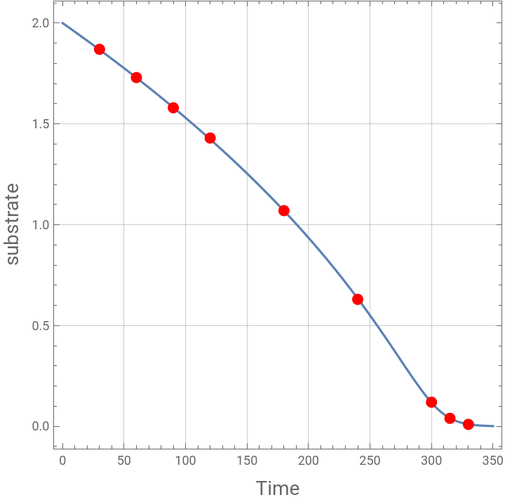
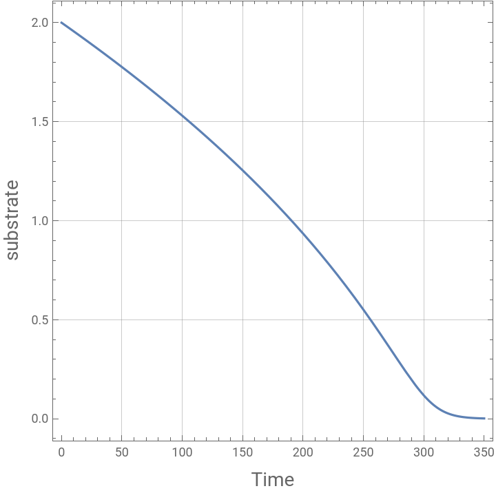
Plotting predicted and experimental values of the substrate concentration versus time. We get perfect agreement.
In[]:=
plt1=Plot[Evaluate[S[t]/.myode[211.184,0.225823,0.522951]],{t,0,350},Frame->True,GridLines->Automatic,AspectRatio->1,FrameLabel->{Style["Time",14],Style["substrate",14]}]
Out[]=
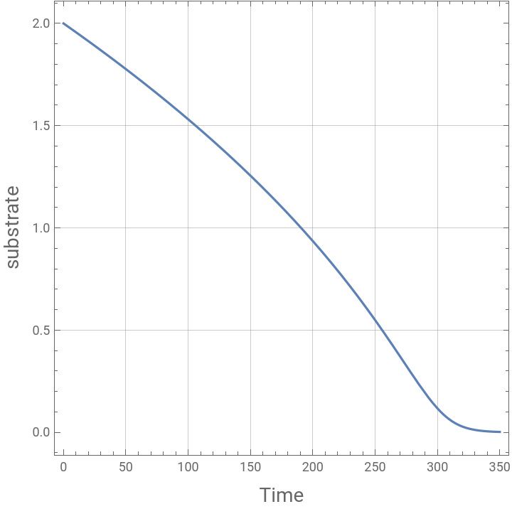
In[]:=
plt2=ListPlot[Table[{time[[i]],sub[[i]]},{i,1,9}],PlotStyle{PointSize[0.025],RGBColor[1,0,0]},Frame->True,GridLines->Automatic,AspectRatio->1,FrameLabel->{Style["Time",14],Style["substrate",14]}]
Out[]=
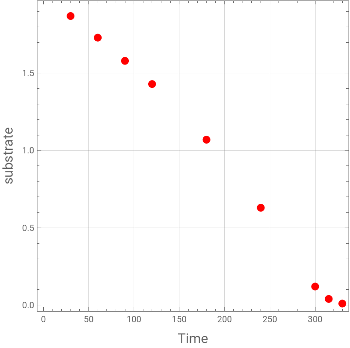
In[]:=
Show[plt1,plt2]
Out[]=
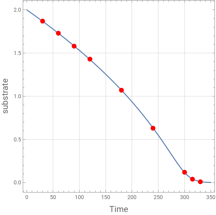
Plotting predicted and experimental values of the substrate concentration versus time. We get perfect agreement for the values found in the textbook by Kenneth Beers using Matlab (Vm=200, Km=0.201 and Ksi= 0.5616).
In[]:=
myode[200,0.201,0.5616]
Out[]=
S[t]InterpolatingFunction[t]


In[]:=
plt3=Plot[Evaluate[S[t]/.myode[200,0.201,0.5616]],{t,0,350},Frame->True,GridLines->Automatic,AspectRatio->1,FrameLabel->{Style["Time",14],Style["substrate",14]}]
Out[]=
In[]:=
Show[plt3,plt2]
Out[]=