The economic model
The economic model
The economic model that we’ll simulate is very simple: each agent, as long as they have resources available, we’ll proceed to give one unit of wealth to another agent at random. way to start into your exposition is to explain how the basic idea works. If it is a formula, provide the math. If it is an algorithm, describe the steps. If it is an experiment, set up assumptions and provide definitions.
Our model will include 400 individuals (agents), starting with 50 units of wealth each. We’ll track each agents wealth across 10^4 units of time (ticks). Let’s create the simulated economy:
Our model will include 400 individuals (agents), starting with 50 units of wealth each. We’ll track each agents wealth across 10^4 units of time (ticks). Let’s create the simulated economy:
In[]:=
nbrOfIndividuals=400;startingWealth=50;individualWealth=ConstantArray[startingWealth,nbrOfIndividuals];ticks=10^4;transactCompiled=Compile[{{individualWealth,_Real,1}},Module[{unitize=Unitize[individualWealth],newWealth,randomPartners,i=1},newWealth=individualWealth-unitize;randomPartners=RandomInteger[{1,nbrOfIndividuals},nbrOfIndividuals];Do[newWealth[[n]]=newWealth[[n]]+unitize[[i]];i++;,{n,randomPartners}];newWealth]]
Out[]=
CompiledFunction


In[]:=
individualWealth=NestList[transactCompiled,individualWealth,ticks];
Wealth Distribution
Wealth Distribution
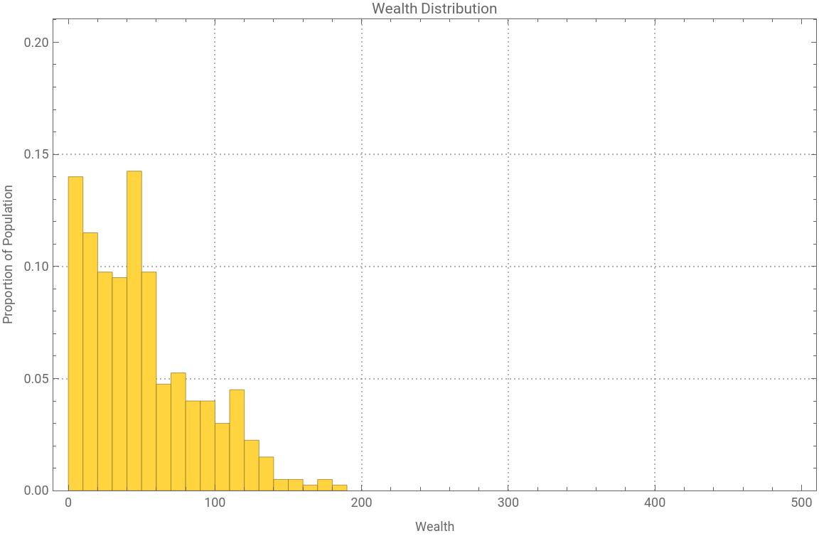
We can explore how the wealth distribution evolves over time. We can observe that the model starts with a uniform distribution, morphs to a student distribution and that finally settles to a Pareto type.
The following code allows to explore how the wealth is distributed among the individuals:
The following code allows to explore how the wealth is distributed among the individuals:
In[]:=
Manipulate[Show[{Histogram[individualWealth[[n]],{0,500,10},"Probability",ImageSizeLarge,PlotTheme"Detailed",FrameLabel{"Wealth","Proportion of Population"},PlotLabel"Wealth Distribution"],ListPlot[{{500,0.2`}},PlotRange{{0,500},{0,1}},PlotStyleWhite]}],{n,1,ticks,10},SaveDefinitionsTrue]
Out[]=


Cumulative Wealth Distribution
Cumulative Wealth Distribution
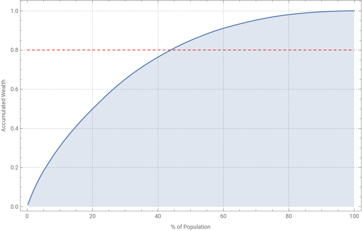
Another interesting aspect of the simulation is to analyze the cumulative distribution of wealth. Let’s explore the last snapshot of the simulation.
We’ll sort the agents by their wealth and observe % of the population that own 80% of the wealth in this simple economic model.
We’ll sort the agents by their wealth and observe % of the population that own 80% of the wealth in this simple economic model.
In[]:=
ListPlot[Transpose[{N[100Range@nbrOfIndividuals/nbrOfIndividuals],Last@individualWealth/(nbrOfIndividuals*startingWealth)//Sort//Reverse//Accumulate}],Epilog{Dashed,Red,Line[{{0,0.8`},{100,0.8`}}]},JoinedTrue,FillingAxis,PlotTheme"Detailed",ImageSizeLarge,FrameLabel{"% of Population","Accumulated Wealth"}]
Out[]=
Social Mobility
Social Mobility
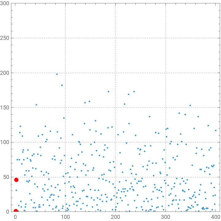
Although the wealth gap remains fairly stable across the simulation run, wealth changes hands across the simulation. The rich of today can become the paupers of tomorrow.
We’ll use the Manipulate function to keep tabs of the economic status of one of the individuals across the simulation epochs.
We’ll use the Manipulate function to keep tabs of the economic status of one of the individuals across the simulation epochs.
In[]:=
Manipulate[ListPlot[{Table[{n,individualWealth[[frame]][[n]]},{n,2,Length[individualWealth[[-1]]],1}],Style[{1,individualWealth[[frame,1]]},PointSize[Large],Red]},AspectRatio1,PlotTheme"Detailed",PlotRange{Automatic,{0,300}}],{frame,1,Length@individualWealth,1},SaveDefinitionsTrue]
Out[]=