The purpose of the project is to explore vector fields and related definitions on the discrete graphs in comparison to definitions on the smooth manifolds. In particular we investigate defining vector fields and scalar fields on graphs programmatically, as well as taking discrete derivations of scalar fields along vector fields and computationally check the relation .
fg+gf+fg==(fg)
∇
x
∇
x
∇
x
∇
x
∇
x
Code
Code
Exploring Vector Fields and Derivations on a Grid
Exploring Vector Fields and Derivations on a Grid
We consider experimenting with the following definitions on the graph:
Definition (Vector Field)
We define vector field on the graph, such that X(v) = w for (v, w) ∈ E thus we have X(v) in the neighborhood of the vertex v, X(v)∈ δ(v). The vertex field assigns each vertex to an outgoing edge.
We define vector field on the graph
X:V->V
For example,
In[]:=
g1=GridGraph[{2,2},VertexLabels->Automatic,EdgeLabels->{1<->2->"X",1<->3->"Y"},ImageSize->100]
Out[]=
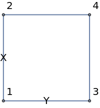
Thus we have ,
X()
v
1
v
2
Y()
v
1
v
3
Definition (Function)
Assume we consider a graph G over a field K. Define function on the graph.
For example,
Assume we consider a graph G over a field K. Define function on the graph
f:VK
For example,
In[]:=
g2=GridGraph[{2,2},VertexLabels->{1->1,2->3,3->8,4->4},EdgeLabels->{1<->2->"X",1<->3->"Y"},ImageSize->100]
Out[]=
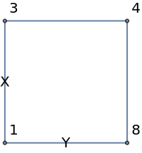
We thus have , , , . ,
f()1
v
1
f()4
v
2
f()8
v
3
f()2
v
4
f(X())f()3
v
1
v
2
f(Y())f()8.
v
1
v
3
Definition (Weight Derivation)
The weighted derivation on the graph satisfies
The weighted derivation on the graph satisfies
D(f·g)fD(g)+D(f)g+D(f)·D(g)
For example, consider , for X in the above graph, which is the derivation with respect to vector field satisfies (f)(v)f(X(v))-f(v),
D
Δ
X
X
Δ
X
Δ
x
v
1
v
1
v
1
v
2
v
1
Δ
Y
v
2
v
1
v
1
v
3
v
1
We can show that this satisfies the condition
(f·g)f(g)+(f)g+(f)(g).
For example,
Δ
X
Δ
X
Δ
X
Δ
X
Δ
X
For example,
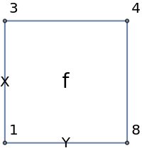
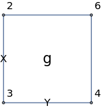
Show[GridGraph[{2,2},VertexLabels->{1->1,2->3,3->8,4->4},EdgeLabels->{1<->2->"X",1<->3->"Y"},ImageSize->100],Graphics[Text[Style["f",14],Scaled[{0.5,0.5}]]]]Show[GridGraph[{2,2},VertexLabels->{1->3,2->2,3->4,4->6},EdgeLabels->{1<->2->"X",1<->3->"Y"},ImageSize->100],Graphics[Text[Style["g",14],Scaled[{0.5,0.5}]]]]Show[GridGraph[{2,2},VertexLabels->{1->3,2->6,3->32,4->24},EdgeLabels->{1<->2->"X",1<->3->"Y"},ImageSize->100],Graphics[Text[Style["fg",14],Scaled[{0.5,0.5}]]]]
·
Out[]=
Out[]=
Out[]=
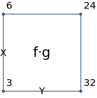
Thus we have (f)()f(X())-f()3-12, (g)()g(X())-g()2-3-1.
(f·g)()(f·g)(X())-(f·g)()6-33
Thus(f·g)f(g)+(f)g+(f)(g)3.
Δ
X
v
1
v
1
v
1
Δ
X
v
1
v
1
v
1
Δ
X
v
1
v
1
v
1
f()·(g)()+(f)()·f()+(f)()·(g)()1(-1)+23+2(-1)-1+6-23
v
1
Δ
X
v
1
Δ
X
v
1
v
1
Δ
X
v
1
Δ
X
v
1
Thus
Δ
X
Δ
X
Δ
X
Δ
X
Δ
X
We can find derivation-preserving operator. For ,∈Der(A), we have ++∈Der(A). For ,, we have ++++.We thus have .Thus we . For example, consider the same graph as before,.
D
1
D
2
D
1
D
2
D
1
D
2
D
1
Δ
X
D
2
Δ
Y
D
1
D
2
D
1
D
2
Δ
X
Δ
Y
Δ
X
Δ
Y
(++)(f)(v)f(X(v))-f(v)+f(Y(v))-f(v)+(f(Y(v))-f(v))f(X(v))-f(v)+f(Y(v))-f(v)+f(X(Y(v)))-f(Y(v))-f(X(v))+f(v)f(X(Y(v)))-f(v)
Δ
X
Δ
Y
Δ
X
Δ
Y
Δ
x
(++)(f)(v)
Δ
X
Δ
Y
Δ
X
Δ
Y
Δ
X◦Y
(++)(f)()f(X(Y())-f()f()-f()4-13
Δ
X
Δ
Y
Δ
X
Δ
Y
v
1
v
1
v
1
v
4
v
1
Suppose we have a graph as below
In[]:=
Show[Graph[{1<->2,1<->3,1<->4,2<->4,3<->4},VertexLabels->Automatic,EdgeLabels->{1<->2->"Y",2<->4->"X",1<->4->"Z",3<->4->"W",1<->3->"V"},GraphLayout->"GridEmbedding",ImageSize->100],Graphics[Text[Style["",14],Scaled[{0.5,0.5}]]]]
Out[]=
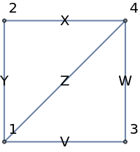
Then we have , which are all vertex fields of the above graph. Thus we have ++ is another derivation over the vector field in the graph.
X◦YZ
X,Y,Z:VV
Δ
X
Δ
Y
Δ
X
Δ
Y
Δ
X◦Y
Δ
Z
If we have a complete graph, such that for any two pairs of vertices in , there are an edge between them,
V
Show[Graph[{1<->2,1<->3,1<->4,2<->4,3<->4,2<->3},GraphLayout->"GridEmbedding",ImageSize->100],Graphics[Text[Style["",14],Scaled[{0.5,0.5}]]]]
Out[]=
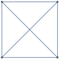
For any vector field we can find . Thus we have
Thus for any we can assign each vertices to any elements in. Thus the equivalent of smooth functions on the graph is for graph with vertices, and in this case above.
However, when our graph is not complete, is no longer surjective.
X,Y∈Vect(G)
X◦YZ∈Vect(G)
Vect(G)≅Der({f:VK}).
Thus for any we can assign each vertices to any elements in
K
n
K
n
4
K
However, when our graph is not complete,
Ψ:Vect(G)Der({f:VK})
Again consider the graph below:
Show[Graph[{1<->2,1<->3,1<->4,2<->4,3<->4},VertexLabels->Automatic,EdgeLabels->{1<->2->"Y",2<->4->"X",1<->4->"Z",3<->4->"W",1<->3->"U"},GraphLayout->"GridEmbedding",ImageSize->100],Graphics[Text[Style["",14],Scaled[{0.5,0.5}]]]]
Out[]=
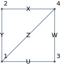
When consider , we can assign any element in in for to be surjective.
However, we do not have much option considering.
Suppose there is, , and thus , . The only vector fields in the neighborhood of are .
Suppose, then we have We have also satisfies the condition, and can be any value in . In this case, . In case, we can consider that are folding the grid the vector field ax an axis.
X◦Y,W◦U
K
Ψ
However, we do not have much option considering
Y◦U,X◦W
Suppose there is
FY◦U
Δ
Y◦U
Δ
F
f(Y◦U())-f()f(F())-f()
v
3
v
3
v
3
v
3
f(Y◦U())f(F())
v
3
v
3
v
3
U,W,0:VV
Suppose
Y◦U0
f()f().
v
2
v
3
X◦W
f(),f()
v
1
v
2
K
dimV
3
K
z
In[]:=
Show[Graph[{1<->2,1<->3,1<->4,2<->4,3<->4},VertexLabels->{1->b,2->a,3->a,4->c},EdgeLabels->{1<->2->"Y",2<->4->"X",1<->4->"Z",3<->4->"W",1<->3->"U"},GraphLayout->"GridEmbedding",ImageSize->100],Graphics[Text[Style["",14],Scaled[{0.5,0.5}]]]]
Out[]=
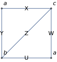
Suppose . Then we have , which we have , or , which we have Suppose . Then we have , which we have , or , which we have In this cases, we are “shrinking “ an edge of the square to form a triangle which is a completed graph.
Y◦UU
f()f()
v
2
v
1
X◦WU
f()f()
v
1
v
3
X◦WY.
Y◦UW
f()f()
v
2
v
4
X◦WW
f()f()
v
4
v
3
X◦WX.
5-5+3
3
K
2
K
1
K
We can then consider pentagon with extra edges
In[]:=
Show[Graph[{1<->2,2<->3,3<->4,4<->5,5<->1,1<->3},(*Pentagonedges*)VertexLabels->Automatic,EdgeLabels->{1<->2->"X",2<->3->"Y",3<->4->"Z",4<->5->"W",5<->1->"U",1<->3->"A"},GraphLayout->{"CircularEmbedding"},(*Ensurespentagonshape*)ImageSize->200],Graphics[Text[Style["",14,Bold],Scaled[{0.5,0.9}]]]]
Out[]=
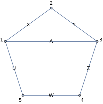
To understand vector fields on smooth manifolds, we aim to further examine a mesh, allowing us to approximate the continuous case. In the mesh, locally, we can see n-gon with an extra vertex in the middle with edges connect to each of the vertices of the n-gon like the following:
This is similar to a (n+1)-gon with some vertices not connected by edges like the following:
Example of RandomGraphVectorField and SmoothGraphVectorField
Example of RandomGraphVectorField and SmoothGraphVectorField
On a Pentagon with a vertex in the middle connecting with all vertices on the pentagon
On a Pentagon with a vertex in the middle connecting with all vertices on the pentagon
On a Complete Graph with 5 Vertices
On a Complete Graph with 5 Vertices
Computing Vector Fields and Derivations on a Discretized Mesh
Computing Vector Fields and Derivations on a Discretized Mesh
Generate Graph for a Discretized Mesh
Generate Graph for a Discretized Mesh
Plot Random Vector Field
Plot Random Vector Field
This random graph does not closely mimic continuous space. For instance, multiple vector fields of neighboring vertices point directly opposite to one another, highlighting inconsistencies. As a result, we want to smooth it out to better mimic continuous space with our discrete graphs.
Smooth Vector Field on Graph
Smooth Vector Field on Graph
Compared to the vector field on the graph, we can see that after a few steps of smoothing, the vector field in the vertex in the center is comparatively much more aligned with the direction of the vector field associated to its neighboring vertices. We can see that it mimic the continuous space much better.
Compared to the vector field on the graph, we can see that after a few steps of smoothing the vector field graph, the vector field in the vertex in the center is comparatively much more aligned with the direction of the vector field associated to its neighboring vertices. We can see that it mimic the continuous space much better.
Derivations
Derivations
On a Pentagon with a vertex in the middle connecting with all vertices on the pentagon
On a Pentagon with a vertex in the middle connecting with all vertices on the pentagon
On a Mesh
On a Mesh
Acknowledgment
Acknowledgment
I am profoundly thankful to Dugan Hammock and Utkarsh Bajaj for setting up the topics and examples, guiding me through the project, and patiently answering my questions. I am also deeply grateful to Xerxes Arsiwalla for providing valuable suggestions to prepare for the winter school, recommending directions for the topics, and helping improve the project. I deeply appreciate Stephen Wolfram and all the speakers for their inspiring talks and discussions during the winter school. Finally, I am immensely grateful to the winter school staff for their efforts in making this an incredible opportunity for learning and exploration!
CITE THIS NOTEBOOK
CITE THIS NOTEBOOK
Exploring vector fields on graphs and their derivations
by Michelle Jing Dong
Wolfram Community, STAFF PICKS, January 16, 2025
https://community.wolfram.com/groups/-/m/t/3358302
by Michelle Jing Dong
Wolfram Community, STAFF PICKS, January 16, 2025
https://community.wolfram.com/groups/-/m/t/3358302