Extractive Distillation of an Equimolar Acetone-Methanol Mixture Using Water
Authors: Housam Binous and Ahmed Bellagi
Extractive Distillation of an Equimolar Acetone-Methanol Mixture Using Water
Authors: Housam Binous and Ahmed Bellagi
Authors: Housam Binous and Ahmed Bellagi
Consider an extractive distillation column operating at atmospheric pressure with 55 stages, a partial reboiler, and a total condenser. It is used to separate acetone and methanol using water as an entrainer (see Ref. 3).
The mixture is assumed to obey the modified Raoult’s law, and activity coefficients are predicted using the Wilson model.
Pure entrainer at is fed to the column at a flow rate equal to at stage 24 (counting from the top). The lower feed is composed of an equimolar mixture of acetone and methanol. The lower feed, at , is located at stage 39 (counting from the top) and has a flow rate equal to .
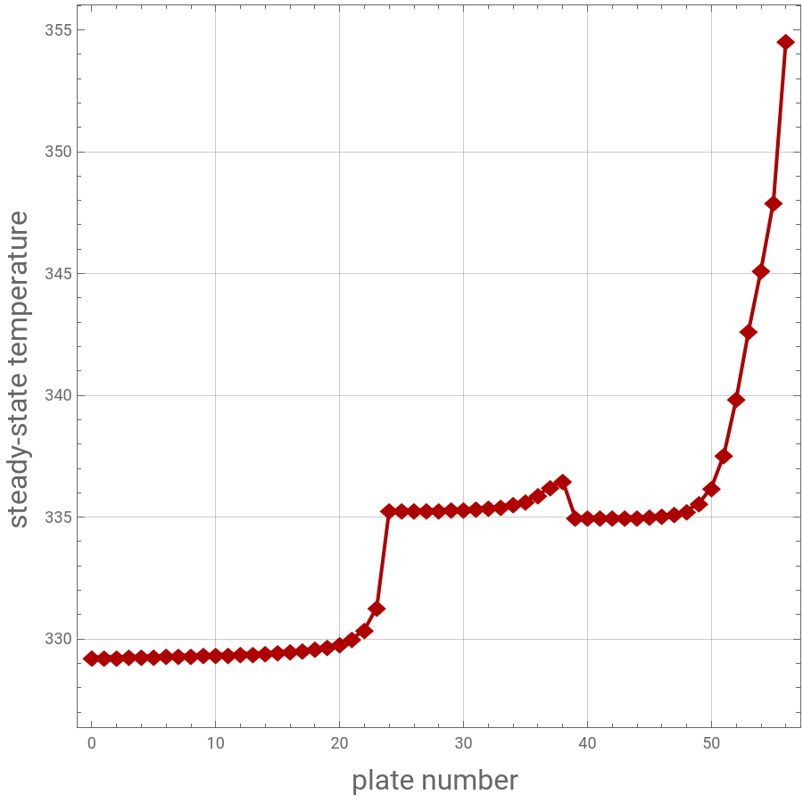
We solve the MESH equations (material, equilibria, summations, and heat) and displays the composition and temperature profiles for a reflux ratio equal to 3.44. The second degree of freedom is set by taking a distillate flow rate equal to. Finally, a comparison of the results of the present calculation with Aspen HYSYS indicates excellent agreement.
The mixture is assumed to obey the modified Raoult’s law, and activity coefficients are predicted using the Wilson model.
Pure entrainer at
320K
1100.03kmole/hr
320K
540kmole/hr
We solve the MESH equations (material, equilibria, summations, and heat) and displays the composition and temperature profiles for a reflux ratio equal to 3.44. The second degree of freedom is set by taking a distillate flow rate equal to
270.7kmole/hr
Constants for the Modified Antoine Equation (obtained from HYSYS)
In[]:=
A1=71.3031;B1=-5952.;C1=0.;D1=-8.53128;E1=7.82393/10^6;F1=2.;A2=59.8373;B2=-6282.89;C2=0.;D2=-6.37873;E2=4.61746/10^6;F2=2.;A3=65.9278;B3=-7227.53;C3=0.;D3=-7.17695;E3=4.0313/10^6;F3=2.;
Expressions of the vapor pressures using the Modified Antoine Equation
In[]:=
PSat[1][i_]:=Exp[A1+B1/(C1+T)+D1*Log[T]+E1*T^F1]/.TT[i];PSat[2][i_]:=Exp[A2+B2/(C2+T)+D2*Log[T]+E2*T^F2]/.TT[i];PSat[3][i_]:=Exp[A3+B3/(C3+T)+D3*Log[T]+E3*T^F3]/.TT[i];
Expressions for the pure components liquid-phase and vapor-phase enthalpies (obtained from Aspen-HYSYS)
In[]:=
a1=0.;b1=135.5999;c1=-8.849995/10^2;d1=9.456661/10^5;e1=1.722499/10^7;h1=a1+b1*T+c1*T^2+d1*T^3+e1*T^4/.T273.15;hl1=a1+b1*T+c1*T^2+d1*T^3+e1*T^4-h1;a2=0.;b2=105.8;c2=-0.1811151;d2=3.126337/10^4;e2=-3.639309/10^13;h2=a2+b2*T+c2*T^2+d2*T^3+e2*T^4/.T273.15;hl2=a2+b2*T+c2*T^2+d2*T^3+e2*T^4-h2;a3=0.;b3=76.28204;c3=2.565142/10^2;d3=-1.127938/10^4;e3=1.325963/10^7;h3=a3+b3*T+c3*T^2+d3*T^3+e3*T^4/.T273.15;hl3=a3+b3*T+c3*T^2+d3*T^3+e3*T^4-h3;a1v=41714.86;b1v=115.8302;c1v=-0.1686754;d1v=2.839015/10^4;e1v=-1.428978/10^8;Hv1=a1v+b1v*T+c1v*T^2+d1v*T^3+e1v*T^4-h1;a2v=50918.36;b2v=93.976;c2v=-0.3743472;d2v=7.937342/10^4;e2v=-6.269264/10^7;Hv2=a2v+b2v*T+c2v*T^2+d2v*T^3+e2v*T^4-h2;a3v=47304.17;b3v=107.5791;c3v=-0.2202581;d3v=3.661611/10^4;e3v=-3.228085/10^7;Hv3=a3v+b3v*T+c3v*T^2+d3v*T^3+e3v*T^4-h3;
Total pressure
In[]:=
P=101.325;
Mixture liquid-phase and vapor-phase enthalpies
In[]:=
H[i_]:=y[1][i]*Hv1+y[2][i]*Hv2+y[3][i]*Hv3/.TT[i];h[i_]:=x[1][i]*hl1+x[2][i]*hl2+x[3][i]*hl3/.TT[i];
Activity coefficients using Wilson Model
In[]:=
Gam[i_,k_]:=Exp[1-Log[Sum[x[j][k]*Aw[i,j,k],{j,1,3}]]-Sum[(x[p][k]*Aw[p,i,k])/Sum[x[j][k]*Aw[p,j,k],{j,1,3}],{p,1,3}]];Aw[i_,j_,k_]:=(Vw[j]/Vw[i])*Exp[-a[i,j]/(R*T[k])];a[1,1]=0;a[1,2]=-124.932800292969;a[1,3]=393.267303466797;a[2,1]=551.454528808594;a[2,2]=0;a[2,3]=-52.6054916381836;a[3,1]=1429.98901367188;a[3,2]=620.631408691406;a[3,3]=0;Vw[1]=7.44767773150726;Vw[2]=4.07621656312461;Vw[3]=1.78833825504182;
Universal gas constant
In[]:=
R=1.987;
Upper-feed and lower-feed temperatures
In[]:=
TFU=320;TFL=320;
Upper-feed and lower-feed enthalpies
hFU=zU[1]*hl1+zU[2]*hl2+zU[3]*hl3/.TTFU;hFL=zL[1]*hl1+zL[2]*hl2+zL[3]*hl3/.TTFL;
In[]:=
y[3][i_]:=1-y[1][i]-y[2][i];x[3][i_]:=1-x[1][i]-x[2][i];
distillate stream enthalpie
In[]:=
h[0]=y[1][1]*hl1+y[2][1]*hl2+y[3][1]*hl3/.TT[0];
Upper-feed and lower-feed flow rates
In[]:=
FU=1100.03;FL=540;
Upper-feed and lower-feed composition
zU[1]=0;zU[2]=0;zU[3]=1;zL[1]=0.5;zL[2]=0.5;zL[3]=0;
Relux ratio
In[]:=
RR=3.44;
MESH equations
In[]:=
eq1=Di+L[0]V[1];eq2=Di*h[0]+L[0]*h[0]V[1]*H[1]+Qc;eq3[i_]:=V[i]+L[i]V[i+1]+L[i-1];eq4[i_]:=Table[V[i]*y[j][i]+L[i]*x[j][i]V[i+1]*y[j][i+1]+L[i-1]*x[j][i-1],{j,1,2}];eq5[i_]:=Table[y[j][i]*Px[j][i]*PSat[j][i]*Gam[j,i],{j,1,2}];eq6[i_]:=V[i]*H[i]+L[i]*h[i]V[i+1]*H[i+1]+L[i-1]*h[i-1];eq7=V[24]+L[24]-FUV[25]+L[23];eq8=Table[V[24]*y[i][24]+L[24]*x[i][24]-FU*zU[i]V[25]*y[i][25]+L[23]*x[i][23],{i,1,2}];eq9=Table[y[i][24]*Px[i][24]*PSat[i][24]*Gam[i,24],{i,1,2}];eq10=V[24]*H[24]+L[24]*h[24]-FU*hFUV[25]*H[25]+L[23]*h[23];eq11=V[39]+L[39]-FLV[40]+L[38];eq12=Table[V[39]*y[i][39]+L[39]*x[i][39]-FL*zL[i]V[40]*y[i][40]+L[38]*x[i][38],{i,1,2}];eq13=Table[y[i][39]*Px[i][39]*PSat[i][39]*Gam[i,39],{i,1,2}];eq14=V[39]*H[39]+L[39]*h[39]-FL*hFLV[40]*H[40]+L[38]*h[38];eq15=V[56]+BL[55];eq16=Table[V[56]*y[i][56]+B*x[i][56]L[55]*x[i][55],{i,1,2}];eq17=Table[y[i][56]*Px[i][56]*PSat[i][56]*Gam[i,56],{i,1,2}];eq18=V[56]*H[56]+B*h[56]L[55]*h[55]+Qr;eq19=L[0]/DiRR;eq20=Di270.7;eq21=Table[Sum[x[i][j]*PSat[i][j]*Gam[i,j],{i,1,3}]P,{j,0,56}];eq22=Table[x[i][0]y[i][1],{i,1,2}];
Solution of MESH Equations using FindRoot
In[]:=
Out[]=
Column temperature profile
In[]:=
ListPlot[{Table[{i,T[i]}/.sol1,{i,0,56}]},PlotMarkers{"◆",16},JoinedTrue,FrameLabel{Style["plate number ",16],Style["steady-state temperature ",16]},FrameTrue,GridLinesAutomatic,PlotStyle{{Thick,RGBColor[0.68,0,0]}},ImageSize{450,450},AspectRatio1,PlotRangeAll]
Out[]=
In[]:=
tblA={0.991585,0.990017,0.988395,0.98673,0.985023,0.983266,0.981446,0.979546,0.977543,0.975409,0.973109,0.970597,0.967816,0.964687,0.961103,0.956911,0.95189,0.945699,0.937784,0.927191,0.912103,0.888602,0.846404,0.747492,0.33043,0.330027,0.329449,0.328649,0.327483,0.325837,0.323508,0.320203,0.315503,0.308765,0.299051,0.285002,0.265154,0.240226,0.222888,0.28688,0.286839,0.286755,0.286596,0.286277,0.285637,0.284339,0.281769,0.276629,0.266478,0.24701,0.21199,0.158092,0.0965697,0.0481618,0.020177,0.00663256,0.00115229};tblM={0.000950239,0.000758714,0.000641417,0.000569825,0.000526424,0.000500449,0.000485282,0.000476846,0.000472637,0.000471119,0.000471357,0.000472792,0.000475105,0.000478133,0.000481823,0.000486211,0.000491413,0.000497644,0.000505257,0.000514826,0.000527315,0.000544428,0.000569288,0.000605859,0.000561091,0.00097198,0.00154956,0.00236189,0.00350492,0.00511481,0.00738482,0.0105902,0.0151244,0.0215493,0.0306631,0.0435717,0.061731,0.0870692,0.124538,0.206163,0.206202,0.206279,0.206433,0.206742,0.20736,0.20859,0.211034,0.215843,0.225149,0.242567,0.272794,0.317333,0.366527,0.402449,0.409975,0.359392,0.196989};tblW=1-tblA-tblM;
Column composition profile (our results versus Aspen-HYSYS results). Excellent agreement between both sets of data is found.
References :
[1] M. F. Doherty and M. F. Malone, Conceptual Design of Distillation Systems, New York: McGraw-Hill, 2001.
[2] E. J. Henley and J. D. Seader, Equilibrium-Stage Separation Operations in Chemical Engineering, New York: Wiley, 1981.
[3] W. L. Luyben and I.-L. Chien, Design and Control of Distillation Systems for Separating Azeotropes, Hoboken, NJ: Wiley, 2010.