We are now ready for a crucial concept : the p - value. You must memorize its definition and understand it. The p-value is a notoriously slippery concept. People misstate its meaning all the time. And they do so in ways that can have catastrophic consequences for research and for the humans it affects. Do not be one of those people.
The first thing to remember is that there are no p-values in the air. The p-value is attached to a statistic and to a test. The test may be legitimate only under certain circumstances and the p-value is only as good as the statistic with which it is associated. Let’s say that again. The p-value is attached to a statistic and to a test. The test may be legitimate only under certain circumstances and the p-value is only as good as the statistic with which it is associated. One more time. The p-value is attached to a statistic and to a test. The test may be legitimate only under certain circumstances and the p-value is only as good as the statistic with which it is associated.
To see what a p - value is, consider the following example. Let’s generate 100 draws from a particular logistic distribution. I’ll call it the null distribution. And let’s do the experiment 10,000 times.
In[]:=
SeedRandom[11102019]
In[]:=
nullDistribution=LogisticDistribution[3,2];
Dimensions[rv=RandomVariate[nullDistribution,{10000,100}]]
Out[]=
{10000,100}
Now, let's compute the same statistic on each of the 10, 000 samples of 100. My statistic will be the median. This gives us a list of 10,000 values.
In[]:=
(medians=Map[Median,rv])//Short
Out[]//Short=
{3.19964,3.38066,9996,3.54773,3.06237}
This list can be used to generate its own statistical distribution. This is NOT the same as the underlying null distribution. It is a derived distribution based on computing a statistic on numerous samples of the underlying null distribution. Read this paragraph until you completely understand it.
In[]:=
medianDistribution=EmpiricalDistribution[medians]
Out[]=
DataDistribution


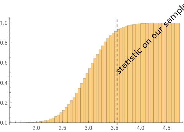
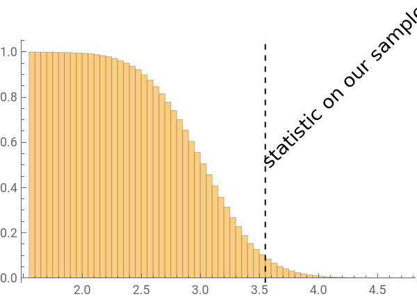
This list can also be used to generate various Histograms that we can then plot. Here I show the “PDF”, “CDF” and “Survival Function” (“SF”) of the median distribution.
In[]:=
Column@KeyValueMap[Curry[Labeled]/*Framed][AssociationMap[hspecHistogram[medians,50,hspec,ImageSize300,BaseStyle14],{"PDF","CDF","SF"}]]
Out[]=
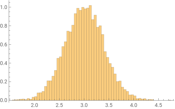
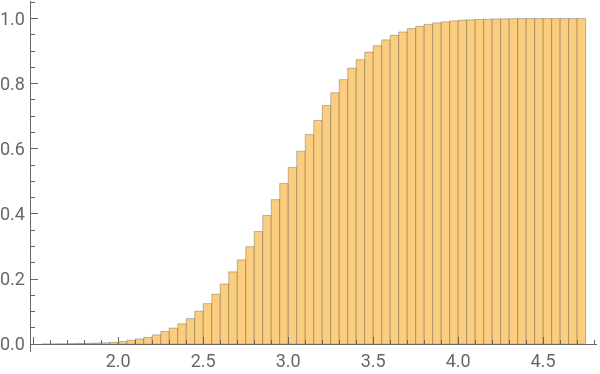
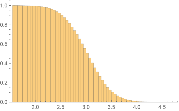
Now, suppose we have some data. Here it is:
In[]:=
sample=,,,,3,,,,,,,,,,,,,1,,,,,,,,,,,,,,,,,,,,,,,,,,,,,,,,,,,,,,,,,,,,,,,,,,,,,,,,,,,,,,,,,,,,,,,,,,,,,,,,,,;
387
100
373
100
207
50
72
25
367
100
527
100
299
100
381
100
163
50
211
100
87
20
139
50
179
50
261
50
79
25
49
25
407
100
353
100
273
50
102
25
187
50
139
50
59
20
94
25
97
25
81
20
31
10
303
100
513
100
253
100
33
25
18
5
339
100
87
25
291
100
47
25
537
100
243
100
219
50
82
25
69
25
189
50
37
10
113
25
461
100
37
10
357
100
371
100
51
20
43
20
191
50
86
25
141
50
291
100
477
100
443
100
433
100
257
100
27
10
249
100
76
25
263
50
109
20
459
100
9
2
481
100
137
50
74
25
383
100
94
25
529
100
169
100
517
100
253
50
83
50
211
100
147
50
33
25
371
100
19
5
237
50
279
100
71
25
17
5
237
100
359
100
167
50
132
25
257
100
403
100
417
100
17
20
291
100
453
100
163
50
323
100
119
25
63
20
Now let' s compute the same statistic on this data as we did on the data from the null distribution.
In[]:=
medianSample=Median[sample]
Out[]=
71
20
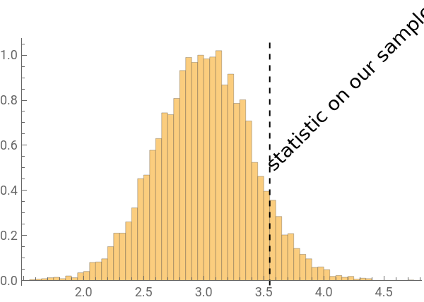
We now ask the big question: how likely is it we would see a statistic resembling the one we do (in a certain way) if the sample data came from the null distribution. I will call this statement “if the sample data came from the null distribution” the null hypothesis.
To figure this out, let's plot out median of the sample on our various histograms. Look at these graphics carefully. They are the most important picture in this essay.
In[]:=
CDF[medianDistribution,medianSample]
Out[]=
0.9166
sampleLineGraphic=GraphicsDashed,Text"statistic on our sample",medianSample,,{-1,0},{1,1},InfiniteLine[{{medianSample,0},{medianSample,1}}];
1
2
Out[]=
One - sided P - values
One - sided P - values
What you can see is that our sample median is on the high side if the data came from the null distribution. But is it implausibly high? I’m now going to annoy you by first showing you the wrong way to proceed because it seems so obviously right that you and others may be enticed by the idea. And in the process I hope to motivate why it is that P-Values are computed in the non-intuitive way that they are.
You might think you could look at the PDF of the median distribution evaluated at our sample median. But this is a problem: there was never an occasion on which the median of our sample was exactly equal to the median of any the list of 100 values in our 10,000 draw experiment.
In[]:=
MemberQ[medians,medianSample]
Out[]=
False
But the problem is deeper that having a discrete distribution for the statistic in question. Maybe we could use some fancy math to derive an expression for the PDF (or other identifying function) of a continuous distribution of the statistic in question. Or, failing that, suppose we ran zillions of experiments so that we ended up for all practical purposes with a continuous distribution for our medians. The code below simulates that process and creates something called a SmoothKernelDistribution.
In[]:=
mediansSKD=SmoothKernelDistribution[medians]
Out[]=
DataDistribution

Here' s a plot of the result.
In[]:=
Show[Plot[PDF[mediansSKD,x],{x,1,5}],sampleLineGraphic]
Out[]=
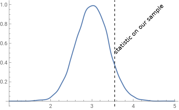
We could now evaluate the PDF of this continuous distribution for the median statistic at the median of our sample.
But what on earth does that number mean? There isn’t any obvious meaning. To see this, suppose our distribution of our underlying statistic was narrowed and our sample statistic had the same CDF value relative to that distribution as our existing sample statistic has to our original distribution.
Here' s the new PDF with the new statistic marked.
Our sample statistic is no more or less probable than it was before. But if we now evaluate the PDF value, here’s what we get:
Nothing fundamental has changed. And yet, we get a completely different number. So, we can’t readily use the PDF in a simple way to figure out anything about how likely it is that we would see the median in our sample if the null hypothesis were true. (There is a very fancy way, but we’re not going there today). Instead, we need to use a different property of the distribution of our median: the CDF (or SurvivalFunction).
Suppose that instead of evaluating the PDF of our median distribution at the value of our sample median, we instead computed the survival function of our median distribution at the value of our sample median. In short, we might compute the fraction of occasions on which the sample median would be greater than our sample median if the data came from the null distribution. The operator we want is > or ≥ and not =. We see that happens 8.34% of the time.
And this value is robust against smushing or spreading of the underlying median distribution. I illustrate this below by doing the same computation but using the smushed median distribution.
That number of 834/10000 has a special meaning : it' s a one - sided P - Value. It' s a P - Value because we are computing a probability of an event given a distribution. And it' s one sided because we are looking only at the probability of values on one side of a particular value.
And so, now you know what a p - value is. Or at least you know that it has something to do with cumulative distributions of a statistic computed if the null hypothesis were true relative to the same statistic computed on the sample data.
A slight digression into statistical significance
A slight digression into statistical significance
I take a slight digression here into the subject of statistical significance. Thus far I have asked about the probability of getting a value as large as something if the statistic in question was derived from the null distribution. But I could ask the inverse question. How large would my sample statistic have to be before the probability of obtaining a value greater than that was less than some “significance level,” say 0.05. That’s the same as asking, in essence, what is the 0.95 quantile of the median distribution.
So, before I could say the sample was different in a “statistically significant” way from that expected by computing the median on the null distribution, I would need to see a sample median of at least 3.6596. And that is true (and only true) if the significance level was set at 0.05.
I could also set my significance level higher. I could set it to 0.01.
If so, I would need to see a sample median of at least 3.95736 before I could say that the difference between my sample median and the sample median drawn from the null distribution would be “statistically significant” at the 0.01 level.
Back to one - sided P - Values
Back to one - sided P - Values
Notice that we computed the probability that the computing the fraction of occasions on which the sample median would be higher than our sample median if the data came from the null distribution. That makes sense because we got a high value of the median for a sample. What if our median was 2.3, however? In that instance, it would likely make more sense to compute the probability that we would see a value as low as 2.3 if the data was generated by the null distribution. We can compute this too.
Here we see there is only a slim chance that we would see a value this low. This is again a one-sided P-Value because we are looking only at the probability of values on one side of a particular value.
Notice that in neither instance is 8.34 % or 3.88 % the probability that the data came from null distribution. We have NO IDEA what that number is. Nor can we say we are 91.66% certain or 96.12% certain that the data did not come from the null distribution. We also have NO IDEA what that number is. When you see people interpreting a P-Value this way, they are wrong, wrong, wrong. They are committing the fallacy of thinking in PDF terms. Also, remember, the P-Value is attached to a statistic. All we can say is that if the data came from the null distribution, we would expect to see a median as large (or small) as the one we have x% of the time.
Two - sided P - Values
Two - sided P - Values
So far I’ve looked at one-sided P-Value statistics. But there are also two-sided statistics. To see this, consider another statistic we could compute : the difference the median of each set of data and the median of the entire data.
Let' s do the same thing of creating a distribution and constructing various Histograms with labels :
Now let' s compute the same median difference statistic on this data as we did on the data from the null distribution.
We can generate decorated Histograms for the new statistic just as I did for the median statistic. Here I show the “PDF”, “CDF” and “Survival Function” (“SF”) of the median difference distribution. Note, by the way, that the distribution appears to be roughly symmetric about zero. I designed my statistic that way deliberately. Generally speaking, we don’t use two-sided P-Values where the distribution of the statistic is not symmetric about some modal value, and usually that modal value is 0.
I could now do the same thing as before and compute one - sided P - Values. But now there is a natural alternative. What if I wanted to compute the probability that one would see a statistic as “extreme” as 0.544797 if the median difference statistic had been generated by the null distribution. To do this, I need a notion of extreme. Here’s one possibility. I look at the difference between my statistic and 0. Equivalently, I want to look at the absolute value of the difference between my statistic and 0. So, what I want is the probability of getting a median difference statistic as large as 0.544797 or as small as -0.544797. Let’s compute this.
So, we could say that if the null hypothesis were true, we would see a median statistic “as extreme” as 0.544797 about 16.53% of the time. And that number 16.53%, is a two-sided value.
Here' s another way to visualize the matter . The red zone represents sample statistics that are farther from the center of the distribution at zero than the negative of our sample median. The blue zone represents sample statistics that are farther from the center of the distribution at zero than our sample median. And the sum of the red and blue areas is equal to the two-sided P-Value.
Here' s yet another way to visualize matters. Here is the CDF of the median difference distribution. The area marked in red are for those values less than the negative of the sample median difference. The area marked in blue are for those values more than the sample median difference. The orange arrow marks the difference between the value of the CDF at the negative of the sample median difference and 0. The purple arrow marks the differences between 1 and the the value of the CDF at the sample median difference . The sum of the lengths of the orange and purple arrows represents a two-sided P-Value.
Some complications
Some complications
If you' ve been following this discussion, you may realize that my definition of extremeness only works sensibly where the PDF of the statistic’s distribution is symmetric about zero. And, indeed, when two-sided P-Values are used, most of the time a statistic is computed whose PDF meets that requirement. One should realize, however, that the two-sided P-Value can be adapted to more complex settings.
Symmetric case
Symmetric case
To see an adaptation of P - Values to symmetric distributions about something other than zero, consider a statistic that computes (for some obscure reason) one plus the difference between the median of the sample and the median of the entire distribution.
Here' s a visualization of the PDF, CDF, and SurvivalFunction of the distribution of the new statistic with the value of the statistic on our sample marked with a line.
Clearly, the distribution is no longer symmetric about zero. But we could proceed exactly as before if we if we transformed our distribution just a tiny bit. Consider a transformed distribution that subtracts a certain number (say 1) from each output of the distribution of our new statistic. We could then proceed exactly as before but work on the transformed distribution. Here’s the code and the picture of the transformed distribution and transformed statistic.
And so the analysis is now exactly the same.
Asymmetric case
Asymmetric case
There' s a more complicated approach that can be taken if the distribution of the statistic is not symmetric. The idea is to again to come up with a definition as extreme. One could compute the CDF of the statistic on the sample relative to the distribution of the statistic. Call one minus that value the “right hand side.” And one could compute the SurvivalFunction of the statistic on the sample relative to the distribution of the statistic. Call that the “left hand side.” The sum of the left hand side and the right hand side is the two-sided P-Value. Perhaps fortunately, this extension is seldom used because two-sided P-Values are generally not used where the distribution of the underlying statistic is not symmetric. Put otherwise, statisticians often try to develop statistics that are symmetric (preferably around zero) precisely so two-sided P-Values can be used.