Topological Kleene Field Theories (TKFTs) represent a new framework in the world of computational theory, where computations are introduced as flows in cobordisms. This project translates this abstract construction intro concrete terms, explicitly computing the smooth dynamics that simulate different Turing machines.
Introduction
Introduction
Topological Kleene Field Theories (TKFTs) are a novel framework recently introduced in [1] that reinterprets the landscape of computation by means of flows on smooth bordisms . By bridging geometry and computation, TKFTs allow computable functions to be understood in terms of dynamical flows and topological decompositions . As discussed by the authors in the paper, this has important implications in the theory of dynamical systems. For instance, it shows that some problems in dynamics, such as determining whether the flow of a point will reach another point or even if the flow will be trapped, are undecidable due to the halting problem. Additionally, they show that the class of vector fields is Turing complete in the sense that any computable function can be simulated by the flow of a field on a bordism.
In the aforementioned article, they way the prove the Turing completeness of this construction is by using the graph representation of a Turing machine. Then, they thicken this graph and by encoding the tape as a
point in the disk through a Cantor set-like embedding, they prove that these simple operations can be implemented using a diffeomorphism. However, the expressions of these diffeomorphisms as well as the explicit cobordisms created using these techniques are not explicitly shown in the paper.
In this project, we have explicitly computed these flows, and hence simulated the computational dynamics on the cobordisms corresponding to certain Turing machines. This explicitly shows that this construction is capable of computing and also helps to better understand the nature of this novel framework of computation.
Computations as dynamics in the Cantor set
Computations as dynamics in the Cantor set
Let us start by understanding how the computations of a Turing machine can be embedded into the Cantor set. An ordinary Turing machine consists on an infinite tape of 1’s and 0’s, which can be represented by cells of two different colors. The computation process is made by a head, which has different states and can move around the tape, reading the symbols and rewriting them. The first important idea of this construction is representing each possible state of the tape (an infinite list of 1’s and 0’s) by a point in the two-dimensional Cantor set.
Embedding the tape into the Cantor set
Embedding the tape into the Cantor set
The first step is two divide the infinite tape into two parts, one first list starting at the position of the head and containing all the digits which are to the right of this position (including the digit the head is currently at), and another list with all the digits to the left of the head. The first list will determine the coordinate in the horizontal Cantor set, while the second part of the tape will be translated into a position in the vertical Cantor set.In order to make this “translation”, one needs to remember that the points in the Cantor sets are those whose ternary expansion consists only on 0’s and 2’s, i.e., only those points in the unit interval which contain no 1’s in base 3. Therefore, if we have a binary sequence , we can define a point in the Cantor set as . If we apply this to our situation, we can read the right and left hand side of the tape as a binary sequence (in the case of the LHS, we read from right to left), and hence transform then into a point in the Cantor set. Using this idea, we can define a function that transforms two lists of 0’s and 1’s into the coordinates of a point in the Cantor set and its inverse, a function that transforms a point in the Cantor set into two lists of 0’s and 1’s.
{}
s
k
k∈
x2
∞
∑
k1
s
k
-k
3
However, although the previous description is more formal and easier to implement computationally, a more intuitive way to understand this embedding is using the iterative definition of the Cantor set. Recall that we can define the Cantor set in an iterative way by taking the interval [0,1] and dropping the middle part, keeping only the first and last thirds. Then, we repeat this process again using these two intervals [0,1/3] and [2/3,1] we just got, dropping the middle part of each of them. The Cantor set is what we get if we repeat this process an infinite amount of time. In order to select a point in the Cantor set, we just need to know if we choose the right or the left part out of the two remaining intervals in each step. The idea of embedding an infinite list of 0’s and 1’s into the Cantor set is based on the fact that every time we read a 0, we choose to keep the left part, while reading a 1 means we get to keep the right part. This way, given an infinite list of 0’s and 1’s we can find the position of the Cantor set just choosing to move right or left.
In the case of the tape of a Turing machine, we have two infinite lists of 0’s and 1’s. The first one, including the place where the head is and everything to its right, encodes the horizontal position, where 0 means left and 1 means right. On the other hand, the left hand side of the tape encodes the vertical direction, and here 0 means down and 1 means up.
Let us use the following tape as an example.
Out[]=
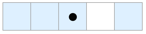
First, we can figure the horizontal position out. We can see that the position where the head is standing is a 1, so we should choose the right third of the whole square. Then, we read a 0, so inside the right column we should choose the left sub-column and then, inside that, we should choose the right part, as the next digit is a 1. The rest of the tape, which is omitted, is a list of 0’s, so we should stay left for the rest of the steps.
Next, we can encode the vertical position. As the two digits to the left of the head are both 1’s, we should choose the upper strip, and inside it, we need to select the upper strip again. Then, we have again that the omitted digits are 0’s, so for the next steps we just stay down. Using these ideas, the final position for this tape is:
Next, we can encode the vertical position. As the two digits to the left of the head are both 1’s, we should choose the upper strip, and inside it, we need to select the upper strip again. Then, we have again that the omitted digits are 0’s, so for the next steps we just stay down. Using these ideas, the final position for this tape is:
Out[]=
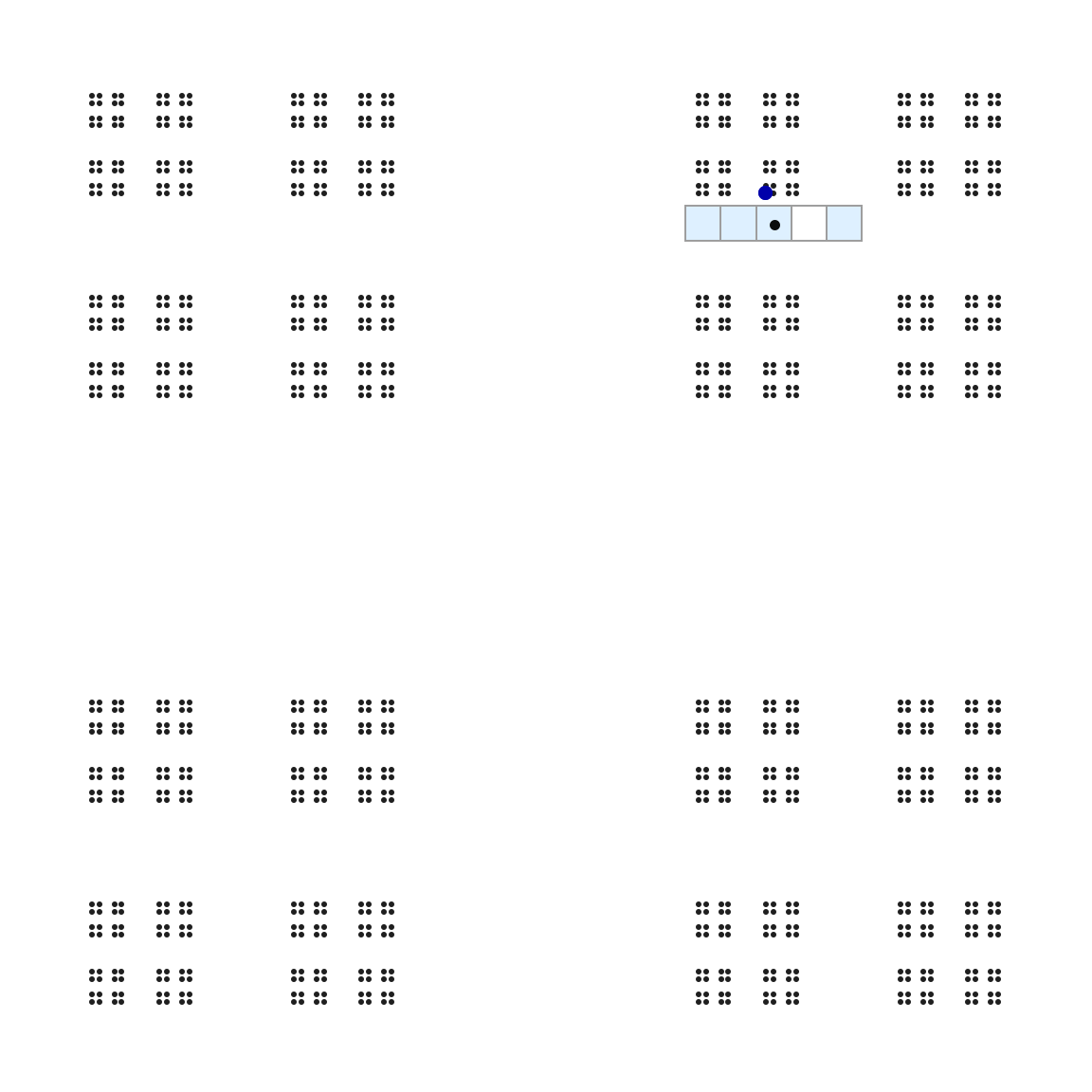
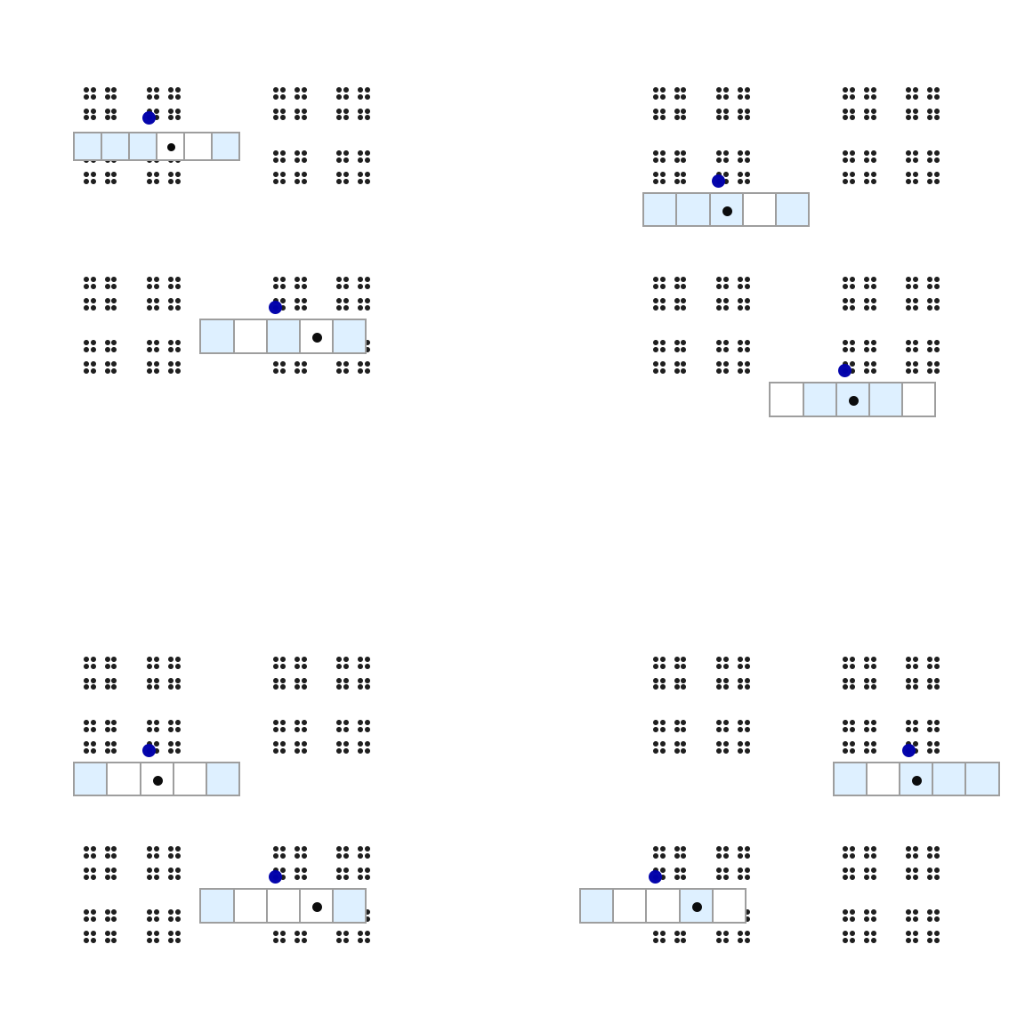
We can check now how different tapes have different positions in the Cantor set:
Out[]=
Turing machine computations as discrete dynamics
Turing machine computations as discrete dynamics
The key idea of this project is that the computation of a Turing machine is equivalent to a dynamical system in the Cantor set. Basically, each step of a computation is changing our tape of 0’s and 1’s to another different tape (while also shifting the position of the head). Therefore, using the language we have developed, each step of the Turing machine is mapping a point in the Cantor set into a different point.
In order to visualize this idea, we can see how the computing process of a complex Turing machine moves a point around the Cantor set:
Out[]=
We can see how the complex behavior of the Turing machine is translated into a very complex discrete dynamical system in the Cantor set.
Flows implementing these computations
Flows implementing these computations
Our next step is to translate these discrete dynamics to smooth flows between two unit squares. The idea is to simulate with these flows the possible actions of a Turing machine: changing the position of the tape and rewriting a symbol; and apply them to all the points in the Cantor set which are affected by them.
Rewriting a symbol
Rewriting a symbol
Let us start with a simple example: rewriting a 0 for a 1. In this case, as the head is reading a 0 the affected tapes correspond to those points in the Cantor set with , which are trivially mapped to the points in the Cantor set with :
x≤1/3
x≥2/3
Out[]=

The flow for changing a 1 to a 0 is analogous:
Out[]=

Shifting the head of the Turing machine
Shifting the head of the Turing machine
The other flows we need are those implementing the movement of the head. We will assume that the head can only move one step to the right or left each time. This movement is equivalent to shifting the tape one step to the left or right, respectively. One can check that taking into account the way we embedded the tape into the Cantor set, performing a right shift of the tape is equivalent to the following piecewise linear map:
R(x,z)=
|
This horseshoe-type map can be extended to a smooth diffeomorphisms of a disk containing the unit square. However, since this extension is not unique, it is hard to explicitly describe and it is not relevant for the computation process, we will only care about its restriction to the upper and lower third of the unit square, i.e., we will only work with the previous map.
We can implement this map as a smooth flow between two unit squares as well, representing the definitions in R with different colors:
We can implement this map as a smooth flow between two unit squares as well, representing the definitions in R with different colors:
The corresponding flow implementing the left shift can be computing using the right shift flow and changing the roles of the horizontal and vertical coordinate:
How Topological Kleene Field Theories work
How Topological Kleene Field Theories work
We can represent it as the following directed graph, where we have included an initializing state and a halting state:
The idea behind Topological Kleene Field Theories (TKFTs) is to thicken this graph so that we can assign a unit square, and in particular a Cantor set, to each of the nodes in the graphs. The computation of the Turing machine will be presented as a smooth flow between these squares. During this computation, the flow will “hit” different squares, each of them associated to the current head state of the Turing machine. The specific position in the square the flow goes through will encode the current state of the tape, using the embedding inside the Cantor set we described in the previous section.
An important remark to be made is that the topology of the manifold we construct plays an important role, and in general it must be nontrivial. This is caused by the fact that sometimes it is necessary to split a certain Cantor set into two branches that diverge, hence creating a nontrivial cobordism with holes in it. Indeed, one can check that the underlying graph that we use as the skeleton of our manifold is a strong deformation retract of the cobordism, so the homology invariants of the manifold, which we can interpret as its “topological complexity”, must be equal to those of the Turing machine graph.
Another important feature of this construction is that these flows are actually generated by a smooth vector field. In particular, this implies that no two trajectories cross each other. In practice, this implies that only reversible Turing machine can be simulated using this method. However, this is not an actual limitation, as any Turing machine can be transformed into a reversible Turing machine by increasing the number of states.
Simulating a 2-state Turing machine
Simulating a 2-state Turing machine
Preliminary definitions
Preliminary definitions
In order to implement this idea we need to define the expressions for the flows between the different disk.
We can also define some graphic elements that will help us visualize the construction better.
Now we are ready to define the function that simulates our 2-state Turing machine:
Simulations
Simulations
Simulating one trajectory
Simulating one trajectory
Let us see now how the evolution of the flow (left) corresponds to the evolution of the Turing machine (right).
Simulating different trajectories
Simulating different trajectories
Now, it is interesting to see how different inputs corresponds to different trajectories and how the same construction works to simulate the computations for any input. We have used different colors to represent these different inputs, representing both, the trajectories in the simulation (left) and the evolution of the corresponding Turing machine (right).
We can see first how the initial position of these trajectories are different and depends on the input of the Turing machine. For example, the blue input is the only one that starts with the head positioned at a 0, and hence it is the only trajectory starting on the left part of the initial square. Then, as we described in the previous case, they all follow different trajectories depending on the computation of the Turing machine for that specific input. For example, the Turing machine halts very quickly for the red input and we can see how the red trajectory is in fact very short. On the other hand, the Turing machine runs for a long time for the black input, and we can check how this corresponds to the black trajectory circling around many times. Finally, we can also visualize how the final position at the halting square of the trajectories depends on the output of the Turing machine for the corresponding input.
Simulating any 3 - state Turing machine
Simulating any 3 - state Turing machine
Our next task will be to create a function that can simulate any reversible Turing machine with three states. This is quite a challenging task. In the previous section we already knew what the graph of the Turing machine looks like, as we had fix the Turing machine beforehand. However, in this section we don’t know a priori how this graph will look like. Therefore, we had to plan ahead and design a way to fit all the possible pipes between states without them colliding with each other.
Layout of the Turing machine
Layout of the Turing machine
How the pipe system works
How the pipe system works
Definitions pipe network
Definitions pipe network
Using these ideas we can define the functions to construct this pipe network.
Examples for different rules
Examples for different rules
Using all these ideas, we can check how the pipe system would like look for some rules.
Let us start with a Turing machine with the following rules:
Let us start with a Turing machine with the following rules:
It is interesting to check that this rules represent indeed a reversible Turing machine.
Now we can check how the the cobordism for this rules look like:
Now we can check how the the cobordism for this rules look like:
In this layout, the closest square to the point of view is the initializing state, while the one that is just behind it is the first state. The rest of squares represent the second, third and halting state, in counterclockwise order. We can check how both pipes exiting the first state go up or down only one “floor” and they both move to the third state. For the pipes exiting the second state, we can see how they move inner into the square and they go up or down two “floors”. Then, the upper pipe goes to the first state (which is the transition coming from a 1), while the lower pipe comes back to the second state. Finally, the pipes exiting from the third states go even deeper into the square. The one coming from a 0 goes down three “floors” and moves to the second state. Meanwhile, reading a 1 in the third state is the halting condition and we can see how the corresponding pipe does indeed goes to the halting state.
If we choose now other rules:
we can see how the cobordism adapts to this rules:
Definitions of the 3-state Turing machine
Definitions of the 3-state Turing machine
Now that we understand the idea of this construction, we can define the functions that will simulate any 3-state (reversible) Turing machine.
We start by defining the expressions for the flow
Definitions of the flow
Definitions of the flow
We will define a flow from each state. This flow will depend on the transition it is simulating, namely, on the state it goes to, the new symbol that it writes and the shift it performs. They also include a halting condition that computes the flow from the particular state to the halting state.
Now we are ready to define the function that simulates any 3-state Turing machine:
Simulations
Simulations
After all this discussion, we are ready to simulate any 3-state reversible Turin machine. For example, we can start with the following Turing machine:
We can try another Turing machine with different rules:
The simulation we get for this case is the following:
Concluding Remarks
Concluding Remarks
This project has taken the first concrete steps toward realizing a Topological Kleene Field Theory as a framework for simulating computation through smooth dynamical systems. By encoding the simulations of a Turing machine as explicit computational flows, we have demonstrated how discrete symbolic computation can be reinterpreted in terms of smooth flows. The fact that we can embed computation into cobordisms and extract its dynamics through flows suggests a promising research direction at the intersection of dynamical systems, category theory, and theoretical computer science.
There is important room for future work. A first natural step would be generalizing the last construction to Turing machines with any number of states. It would be also interesting to further understand and visualize the structure of the vector fields associated with the flows. Finally, one next step into developing the theoretical framework would be to analyze the dynamics for points outside the Cantor set, and explore if they can be used to improve the computations.
There is important room for future work. A first natural step would be generalizing the last construction to Turing machines with any number of states. It would be also interesting to further understand and visualize the structure of the vector fields associated with the flows. Finally, one next step into developing the theoretical framework would be to analyze the dynamics for points outside the Cantor set, and explore if they can be used to improve the computations.
Acknowledgments
Acknowledgments
◼
To my mentor, Dugan Hammock, for all his help during these three amazing weeks at the Wolfram Summer School.
◼
To Ángel González-Prieto, Eva Miranda ad Daniel Peralta-Salas, who have supported me enormously, believing in me and giving me incredible opportunities during the last few years.
◼
To Stephen Wolfram, for the wonderful conversations about my project and his priceless suggestions on how to approach and improve this exposition of TKFTs.
◼
To all the staff and my colleagues at the Wolfram Summer School who have not only helped me many times when preparing this project, but who have also made this summer school an unforgettable experience.
This article has been partially supported by the project reference PID2023-146936NB-I00 financed by the Spanish State Agency MCIN/AEI/10.13039/501100011033/ FEDER, UE.
References
References
1
.Á. González-Prieto, E. Miranda and D. Peralta-Salas (2025), “Topological Kleene Field Theories: A new model of computation”, Preprint arxiv. https://arxiv.org/abs/2503.16100
2
.C. Moore (1990), “Unpredictability and undecidability in dynamical systems”, Physical Review Letters. https://sites.santafe.edu/~moore/nonlinearity-gs.pdf
3
.Stephen Wolfram (2002), “A New Kind Of Science”, Wolfram Media,https://www.wolframscience.com/nks/
Cite This Notebook
Cite This Notebook
Computation through smooth dynamics: simulating TKFT's
by Isaac Ramos
Wolfram Community, July 9, 2025
https://community.wolfram.com/groups/-/m/t/2959123
by Isaac Ramos
Wolfram Community, July 9, 2025
https://community.wolfram.com/groups/-/m/t/2959123