We can use the Wolfram Models to represent space as the large-scale limit of a spatial hypergraph, and spacetime as the large-scale limit of a causal graph. Furthermore, concepts like a ‘frame of reference’ and constants like the speed of light, c, arise rather naturally or as a direct consequence of the models. Given that we can effectively model such fundamental concepts, we are led to question if it is possible to describe General Relativity phenomena using the Wolfram Models. Phenomena including Black Holes, Event Horizons, and Timelike and Spacelike Singularities.
But how can we describe a Black Hole in terms of the Wolfram Models? Mathematically, a Black Hole is defined as a region of Spacetime where events occurring outside the region can affect events occurring inside it. While events occurring inside the region cannot affect events happening outside it. We can think of such unidirectional causal relationship in simpler terms; things can go into the Black Hole but cannot go out of it. Once something crosses the Black Hole’s Event Horizon, it is ‘trapped’ inside and directed towards the singularity.
We can then look for Black Holes by looking for such unidirectional Causal Structure. Applying the function “CausalConnectionGraph” will output such relationships.
For instance, the rule {{{1,1,2},{3,4,2}}{{4,4,2},{4,3,1},{5,3,2}}} produces the following causal graph after 10 steps:
In[]:=
ResourceFunction["WolframModel"][{{{1,1,2},{3,4,2}}{{4,4,2},{4,3,1},{5,3,2}}},Automatic,10]["LayeredCausalGraph",VertexLabelsAutomatic]
Out[]=
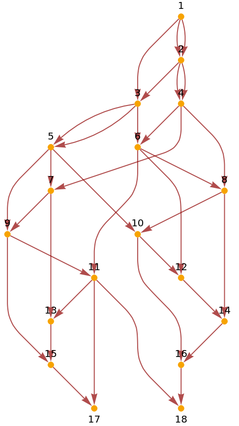
We can assess its Causal Structure applying the function “CausalConnectionGraph”:
In[]:=
ResourceFunction["CausalConnectionGraph"][Function[{layer},WolframModel[{{{1,1,2},{3,4,2}}{{4,4,2},{4,3,1},{5,3,2}}},Automatic,layer,"CausalGraph"]],5,10,VertexLabelsAutomatic]
Out[]=

As mentioned before, the unidirectional causal relationship means that the future of event 7 can affect the future of even 8, but not the other way around. Such behavior is clear once we trace the future of both events and compare the overlap:
We can assess its Causal Structure applying the function “CausalConnectionGraph”:
In[]:=
blackHolePlot[rule_,steps_]:=(With[{gg=Graph[ResourceFunction["WolframModel"][rule,Automatic,steps]["LayeredCausalGraph",VertexLabelsAutomatic]]},HighlightGraph[gg,{Style[Subgraph[gg,VertexOutComponent[gg,#,steps]],Red,Thick]},ImageSize300]]&/@VertexList[ResourceFunction["CausalConnectionGraph"][Function[{layer},WolframModel[rule,Automatic,layer,"CausalGraph"]],5,10]][[All,1]])
In[]:=
blackHolePlot[{{{1,1,2},{3,4,2}}{{4,4,2},{4,3,1},{5,3,2}}},10]
Out[]=
,
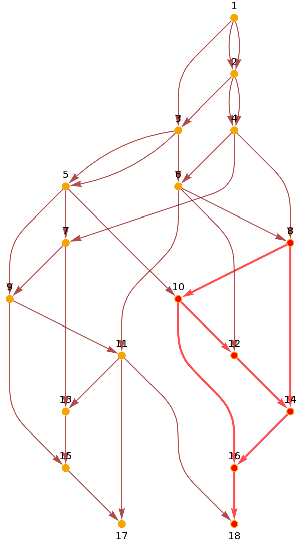
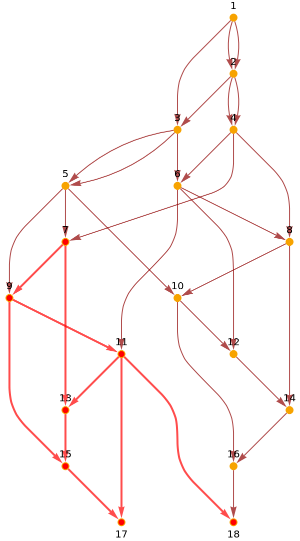
The future of 7 includes the left-hand side of the graph (vertices 9, 11, 13, 15, 17, 18). While the future of 8 includes the right-hand side of the graph (vertices 10, 12, 14, 16, 18). The right-hand side of the graph represents a Black Hole, the future of events occurring inside it cannot affect events happening outside, but the future of events occurring outside can affect the inside (e.g. 5 -> 10, 11-> 18). Furthermore, starting on event 4, you can either cross the event horizon (vertex 8), and “fall into the Black Hole,” or escape and affect the rest of the universe.
Nevertheless, that Black Hole “behavior,” tends to disappear after a few steps for many rules, including the present example:
Let us examine the graph’s Causal Structure, this time after 11 instead of 10 steps:
In[]:=
ResourceFunction["CausalConnectionGraph"][Function[{layer},WolframModel[{{{1,1,2},{3,4,2}}{{4,4,2},{4,3,1},{5,3,2}}},Automatic,layer,"CausalGraph"]],5,11,VertexLabelsAutomatic]
Out[]=
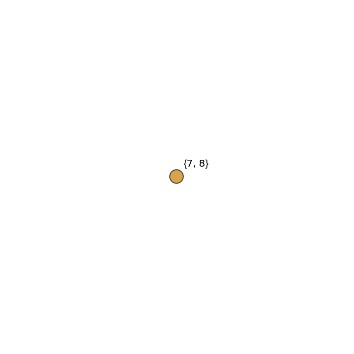
There is no longer a unidirectional relationship, and both vertices 7 and 8 lead to completely overlapping futures.
When looking at the Causal Graph:
In[]:=
blackHolePlot[{{{1,1,2},{3,4,2}}{{4,4,2},{4,3,1},{5,3,2}}},11]
Out[]=
,
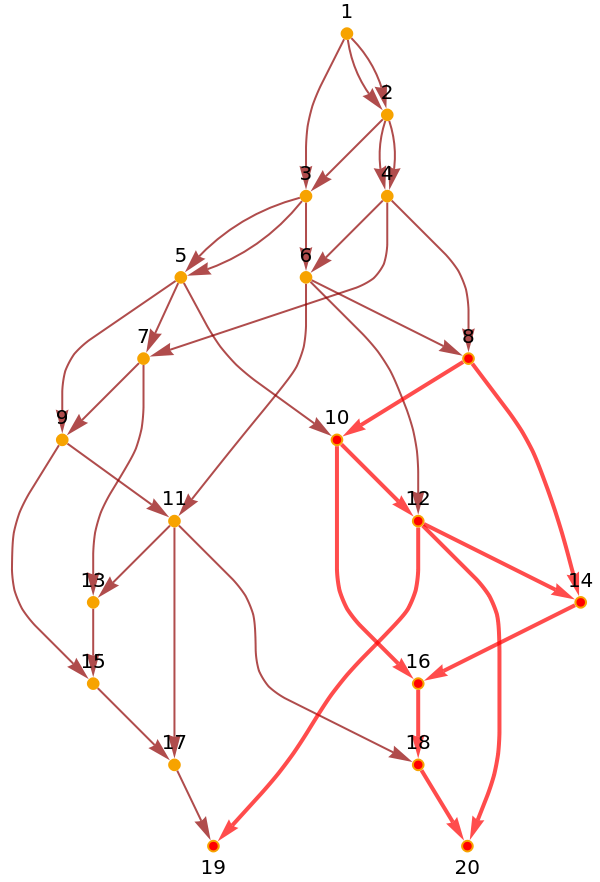
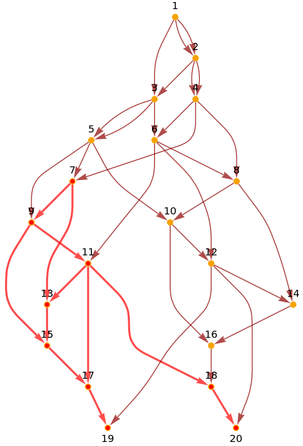
Events inside and outside the Black Hole lead to the same future (events 19 and 20). Events happening inside the Black Hole are able to affect events on the outside of the Black Hole, which means that it has disappeared.
Finding Black Hole Examples
Finding Black Hole Examples
Along the same lines, we can now design a function which checks for the Causal Structure of the graph after a certain number of steps, looks for unidirectional causal relationships and outputs a Boolean value. Where “True” means there is a Black Hole, and “False” means there is not:
In practice, the function gets the Causal Connection Graph, and extracts all the edges. If there is a Black Hole (or nested Black Hole) the list will not be empty. There is no Black Hole otherwise:
In[]:=
causalConnectionGraph[rule_,{startLayer_,endLayer_},o:OptionsPattern[]]:=ResourceFunction["CausalConnectionGraph"][Function[{layer},WolframModel[rule,Automatic,layer,"CausalGraph"]],startLayer,endLayer,o]
In[]:=
blackHoleQ[rule_,{startLayer_,endLayer_}]:=EdgeList[causalConnectionGraph[rule,{startLayer,endLayer}]]=!={}
We can test the function over the previous example, after 10 steps:
In[]:=
blackHoleQ[{{{1,1,2},{3,4,2}}{{4,4,2},{4,3,1},{5,3,2}}},{5,10}]
Out[]=
True
The function recognizes there is a unidirectional causal relationship, a Black Hole. And if we check after 11 steps:
In[]:=
blackHoleQ[{{{1,1,2},{3,4,2}}{{4,4,2},{4,3,1},{5,3,2}}},{5,11}]
Out[]=
False
As expected, the Black Hole “disappears.”
Visualizing Black Holes
Visualizing Black Holes
Furthermore, it is useful to visualize both the inside and outside of the Black Hole on the same graph. We design a function for that:
Testing the function on our previous example:
Where the interior of the Black Hole is drawn in black and exterior in orange.
It is insightful to visualize where in the hypergraph the events related to the Black Hole occur. To do that, we can create another function which highlights the nodes and edges “edited” by the events in the Black Hole:
Testing the function on our previous example:
Applying blackholeQ and blackHolePlots:
Applying blackholeQ and blackHolePlots:
Furthermore, we can apply our Black Hole query function to any list to Wolfram Rules to find Black Hole examples.
First, we tested all 947 rules in the Registry of Notable Universes. It is important to note that it is highly computationally expensive to run the function over long lists. In the case of the present project we ran the function over parts of 100 rules each. Still, a few of the rules were particularly computationally expensive to run, requiring us to run the function over smaller part (50 and 10 elements long).
Out of the 947 rules, 62 led to unidirectional causal relationships within the first 10 steps. However, and as we explored before, we expect many of the Black Holes to “disappear” rather quickly, which is why we then tested those rules again, this time after 12 steps. Out of the 62 rules, only 36 Black Holes “survived.” We tested the list of rules a few more times, and at the end we found 21 rules that lead to Black Holes who survive at least until step 25 (20 steps after the creation of the Event Horizon).
These are the corresponding 21 rules for the surviving Black Holes:
We can now plot their causal graphs. As before, all Black Hole interiors are colored black. Note that some systems include more than one Black Hole.
We proceed to plot their spatial graphs:
Black Hole Dimensionality Analysis
Black Hole Dimensionality Analysis
An interesting question that arises is whether the interior and exterior of the Black Hole present different spatial dimensions. We can check this by creating a new function, “BHdimensionalities” will output a list of the calculated dimensionalities (from different starting points), which we can then plot into a Histogram to see any emergent dimensionality trends:
It is useful to plot the causal and spatial graphs alongside the histogram. Moreover, note that the black bars in the histogram correspond to the interior of the Black Hole while the orange ones represent its exterior:
Our analysis does not show any significant dimensional difference between the exterior and interior of the Black Hole. However, it is important to note that the Black Holes examples we worked on does not accurately represent our notion of the interior of a Black Hole. More specifically, in many most of our examples there is constant Spacelike expansion and Timelike progression, which most certainly lead to the interior of the “Black Hole” to present similar dimensions than the exterior of the region.
Some other examples:
Future Work
Future Work
Although we have not found an accurate representation of a Schwarzschild Black Hole (where the whole interior of the Black Hole winds up at a single Spacelike Singularity, we were able to develop useful functions for its search. It is crucial to keep working on the subject, develop some intuition over the kind of initial conditions that are likely to lead to such structure, and find the specific rule that models it. Once we are able to find an accurately described Schwarzschild Black Hole, it will be relevant to run the dimensionality analysis over it, as differences between the interior and exterior of the region could be significantly different as the spatial expansion and time progression will certainly be different.