Black holes are the most extremal gravitational objects. More than 100 years after the publication of the first Schwarzschild solution, we analytically understand the uncharged, rotating Kerr solution, which is the standard model for astrophysical black holes. Nonetheless, theoretical results have historically been counterintuitive: even Einstein himself initially wrote that the Schwarzschild black hole cannot form in nature. Particularly, the behaviour of light, and how our perception of reality is shaped near a black hole, is rarely explained thoroughly or depicted accurately. In this computational essay, we use the Wolfram Language to model gravitational lensing and review the core principles behind images like Interstellar’s Gargantua.
How do we “see” black holes?
How do we “see” black holes?
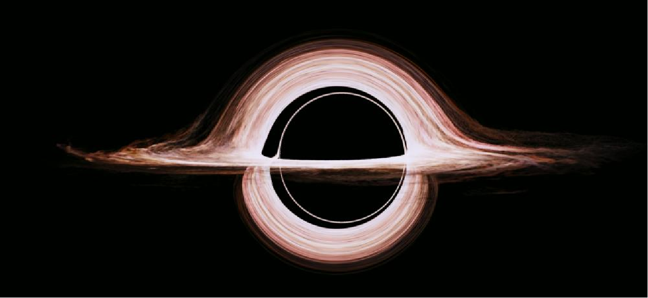
Accretion disk modelled by the Double-Negative artists and gravitationally lensed by a spinning black hole, taken from [1].
In 2014, the movie Interstellar shook the world with beautiful black hole renders. Following the scientific advice from Kip Thorne, the Double Negative team produced what is widely considered the most scientifically accurate and visually groundbreaking black hole simulation in the history of cinema. Five years later, the Event Horizon telescope collaboration made headlines worldwide with the images of Messier 87. Using 8 worldwide synchronized radio telescopes pointing at the centre of a galaxy, the collaboration managed to produce a real image that matches our predictions based on General Relativity.
In this computational essay, the main aim is to understand the core principles behind black hole images. To achieve this, our approach is primarily visual and pedagogical, aimed at a more general audience. For the theoretical details, numerous resources already contain explanations on how to produce these visualizations and compute the light trajectories, see e.g., [2, 3, 4]. Instead, our focus will be on uncovering the core principles by abstracting the involved mathematics away, and providing simple explanations with graphics and pictures.
Throughout the text, we measure degrees in radians, and fix the constants G = c =1.
Gravity bends light
Gravity bends light
Classically, black holes emit no light. So how do we “see” them? We must consider how these interact with the objects surrounding them. In particular, we need to determine the paths of light rays from objects around the black hole towards our telescopes or our own eyes.
General Relativity (GR) predicts how matter and light rays interact with gravitational sources. In contrast with the Newtonian paradigm based on forces acting on objects, GR models these trajectories via the notion of curvature. The Einstein equations tell us how mass concentrations bend space and time, and the curved space and time tells matter and light how to move. Within GR, the fundamental object that encodes the description of space and time is called the metric, which serves as a ruler for measuring distances between two different points in space and time. Once we choose some coordinates to describe our metric, the relative distances between space and time describe the curvature of where all the Physics occurs, what we call the background.
The Schwarzschild solution (1918) describes the spacetime around a spherically symmetric concentration of mass M that does not change with time( i.e., it is stationary). The corresponding metric can be written as
Out[]=
2
d.s.
2
d.r.
1-
2M.
r.
2M.
r.
2
d.t.
2
r.
2
d.θ.
2
r.
2
d.ϕ.
2
Sinθ.
Above, t ∈ (-∞, ∞) is the coordinate time, θ ∈ (0, π) is the polar angle, ϕ ∈ (0, 2π) is the azimuthal angle and r ∈ (2M, ∞) is the radial distance to the origin. The triad {r, θ, ϕ} corresponds to the usual conventions on spherical polar coordinates. At r = 2M we have the event horizon, a special place where this form of the metric, in terms of the {t,r,θ, ϕ} coordinates, breaks down. Once light, or anything, crosses the event horizon, it cannot escape. This is hinted at by the divergence of the coefficient of the -factor for r = 2M. As you can observe, writing the the metric coefficients inside a 4x4 matrix, we have
2
dr
Out[]//MatrixForm=
-1+ 2M. r. | 0 | 0 | 0 |
0 | 1 1- 2M. r. | 0 | 0 |
0 | 0 | 2 r. | 0 |
0 | 0 | 0 | 2 r. 2 Sinθ. |
so these do not depend on t, i.e., the metric is stationary, nor do they depend on ϕ, i.e., the metric is axisymmetric. This implies that both the energy and the angular momentum of the spacetime will be conserved.
Making use of the metric, we can compute the trajectories of massive objects and light around the black hole, called geodesics. As we are interested in how light interacts with black holes, our focus will be on a specific type of geodesic: null geodesics, which describe the path of light rays or photons around the black hole. Typically, to compute these geodesics we solve the geodesic equations, a set of coupled second order ODEs which will give us how the coordinates {t,r,θ, ϕ} change along the geodesic, as we traverse it following a parameter λ. See [2,4] for details.
Instead of focusing on the algebra, let us produce visuals to understand the qualitative picture. For starters, we reduce the complexity of the problem looking on the Schwarzschild spacetime from above, i.e. we focus on the θ = π/2 or equatorial slice of the spacetime. Our final goal is to understand what we would see if we were standing close to a black hole, but far enough to avoid falling in and to remain stationary outside. Computationally, we are only interested in the light rays that reach us, not all of the light rays coming from all the directions in spacetime. As geodesics do not care about which direction we pick to traverse them, we can choose to parametrize our geodesics in a reverse order: start at our eye or camera, and follow them backwards to see where they came from.
Let us represent the black hole event horizon with a dark disc of radius r = 2M and the photon sphere with a gray disc of radius r = 3M. The photon sphere denotes the closest distance where light can orbit around the black hole in perfect circles, any perturbation from there will send the photons either to r ∞ or to plummet into the black hole. Representing the observer (us) with a red dot, and the light path with a yellow trajectory, the top view of the path of a light ray that reaches us a large distance is given by
Out[]=
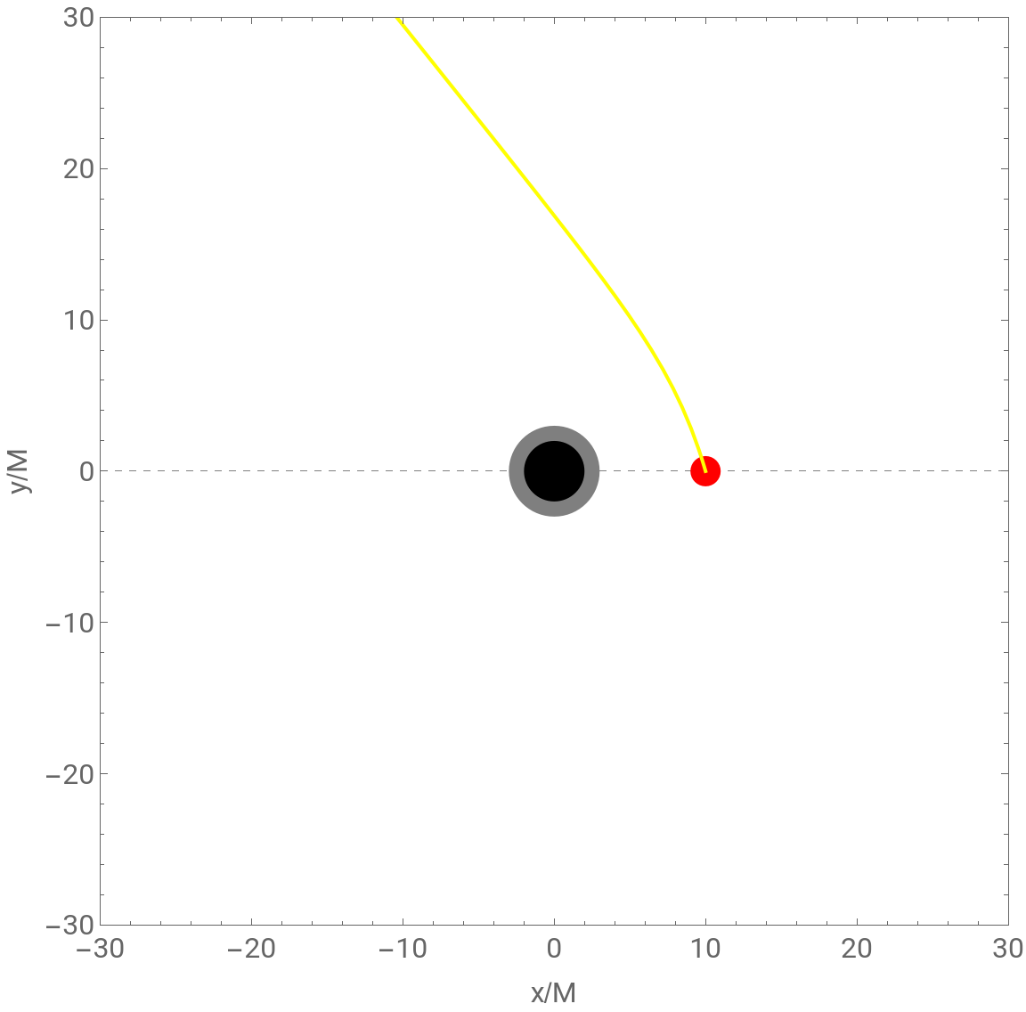
Notice that for numerical convenience, we measure all the quantities in units of M. When doing the computation, this is equivalent to setting M =1, so that the event horizon is at r = 2 and the photon sphere at r = 3 (and θ = π/2 for both). One of the most striking things that you can observe immediately is that, indeed, light follows a curved path. This is counterintuitive, as in our day-to-day experience, we assume that light rays follow straight line paths. Indeed, when gravity is weak (for GR standards anyway, that is why Newtonian theory allowed us to put a spaceship on the moon!) there is no curvature, and light DOES travel following straight lines. The geodesics of flat spacetime are straight lines. We can see this if we position ourselves far enough from the black hole:
Out[]=
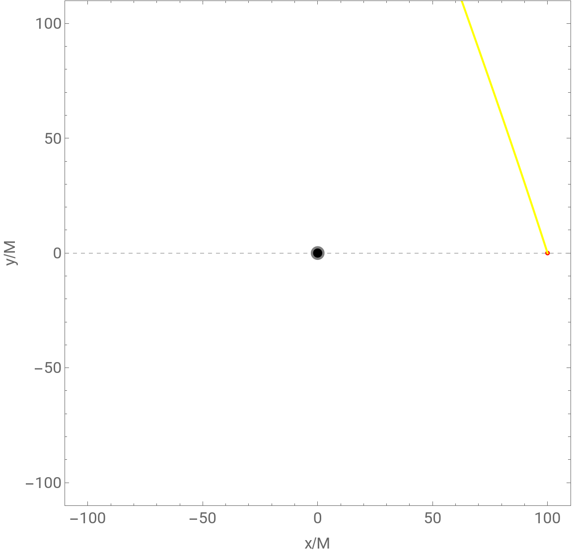
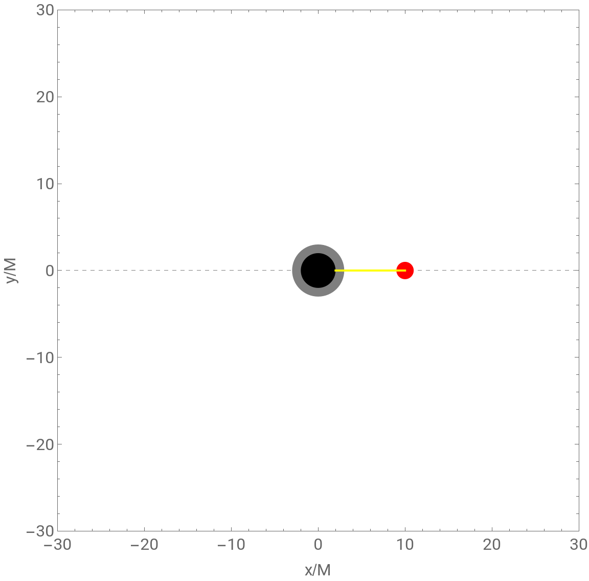
So light no longer cares about the black hole. The choice of angle at which light leaves the camera conditions the result. If we were to stare into the black hole, we can trace a light ray backwards and confirm that.
Out[]=
How do we see the rainbow?
How do we see the rainbow?
Lensing an image
Lensing an image
Hot matter swirling around black holes: accretion disks
Hot matter swirling around black holes: accretion disks
The inner radius will be fixed at 15 M, for all of our visualizations.
Putting a spin on it
Putting a spin on it
Light paths around a spinning black hole (Kerr)
Light paths around a spinning black hole (Kerr)
The squeezing of the shadow
The squeezing of the shadow
Hot matter swirling around a Kerr black hole: accretion disks
Hot matter swirling around a Kerr black hole: accretion disks
CITE THIS NOTEBOOK
CITE THIS NOTEBOOK