Introduction
Introduction
A long time ago I began a series of ‘computational lectures’, designed to introduce students (or other interested parties) to topics that they hadn’t seen before. This is the third installment, looking at Polar coordinates.
Early on in school (I hope) you will have learnt about Cartesian coordinates, although nigh-on all institutions will just teach you about ‘coordinates’. Hopefully you will agree that they’re quite intuitive: you have two axes, and the distance along each is given by a set of coordinates, in the form of (x,y). A more rigorous definition of the point defined by that (x,y) is that we subtend a vertical line from the point x-units from the origin (where the axes intercept), along the x-axis, and a horizontal line from the point y-units from the origin, along the y-axis. Where those two lines intercept is the true point that (x,y) gives.
Of course, we can do this as easy as pie after barely any practice. What I am trying to show you is that, when written down, the simplest of things might seem more complicated - eventually Polar coordinates will seem as easy to you as those in the Cartesian form.
What you’ll find, in fact, is that coordinate systems are more similar than you expect. We can draw some nice parallels between the Cartesian and Polar systems (especially using the Wolfram Language, which is great for this kind of maths) to make the learning journey quite smooth. A last point - I’m not sure what level this ‘lecture’ can be considered for. Polar coordinates are introduced at wildly different times in different syllabi, and also in different ways. Generally speaking they will appear from around a year below undergraduate level, but often not in much depth - so read on to see if this will be useful for you! We start off here by looking at points, progress onto lines and circles, then to more complicated (and interesting!) graphs, and then for a short sojourn in three-dimensions. That last one is very rare to meet before a degree, and we’re going to cover them all at a pretty fast pace - hence why this can be considered a break-neck guide to Polar Coordinates for the Wolfram Language.
One quick note - as is always the case in maths, although this may seem pointless, being another coordinate system to remember and convert between, it is not. Later we’ll see how very simple Polar curves can create the most wonderful graphs, that even seasoned mathematicians would dislike in their Cartesian form.
Points in the Polar Plane
Points in the Polar Plane
Rather than spending time aimlessly meandering about the point (pun unintended), let’s dive right in. Polar coordinates use, put simply, the fact that any point can be uniquely identified (note that that is vital for coordinate systems) by:
- Their distance from the origin
- The angle a straight line from the origin to the point makes with the positive x-axis.
That might seem a bit abstract: here’s an example. The point (2,2) on a Cartesian plane has distance from the origin, by Pythagoras’ Theorem ), noting that a in this case is the direct distance from the origin. Let’s plot it quickly using the Wolfram Language:
- Their distance from the origin
- The angle a straight line from the origin to the point makes with the positive x-axis.
That might seem a bit abstract: here’s an example. The point (2,2) on a Cartesian plane has distance from the origin
2
2
(=b^2+c^2
2
a
Combining two plots to show our point and the line connecting it to the origin.
In[]:=
p1=ListLinePlot[{{0,0},{2,2}}];p2=ListPlot[{{2,2}}];Show[p1,p2]
Out[]=
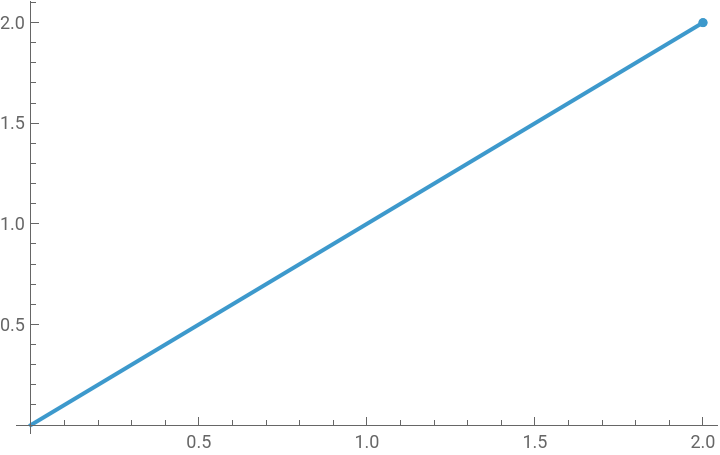
So you can see the point at the end of the ‘imaginary’ line. The distance, as shown, is , and we can consider the angle from the line to the positive x-axis quite easily. In fact (as the coordinates are the same) we have tan(θ)= 2/2 = 1. You could put that into your calculator, but hopefully you’ll know it: it’s 45 degrees.
Now that we know the distance and angle, we’ve got our Polar coordinate: we can just say that it’s, ). Unfortunately, that’s wrong - the reason is our use of degrees, when we should be in radians.
2
2
Now that we know the distance and angle, we’ve got our Polar coordinate: we can just say that it’s
(2
2
o
45
Radians
Radians
I was almost tempted to skip this section, as I was certain you will be aware of this, but once again this is something people can encounter at different times. Feel free to skip ahead if you feel confident with Radians already.
Now, we’ve looked at alternative coordinate systems: there are also alternative angle systems. You might have seen them while browsing your calculator’s settings. Vitally, radians make use of π, or pi. The key idea is that π radians (or, or even π rad) is equivalent to . Radians come in very useful at higher-level mathematics, which is why (generally speaking) at those higher-levels radians will always be assumed to be used.
Setting π radians tomight seem arbitrary from the start. What’s actually going on is that we’ve let be equal to the angle of a sector that has an arc of length 1, for a unit circle (alternatively, the length of the radius for the circle).
In case sector and arc have been forgotten by you, remember that a sector is like a pizza slice of a circle, whereas an arc is the bit on the outside (the crust, if you’d like to continue with the previous analogy).
Now, bear with me. The total circumference of a unit circle (radius 1) will be 2π, as the circumference is given by 2*π*r. I won’t delve into it any further here, but a quick calculation yields the excellent radians = 180 degree.
Think a little of that. What you might see is that we can therefore convert into radians by dividing by 180 and multiplying by π, and vice versa we can convert from radians into degrees by multiplying by 180 and dividing by π. We can now return to our previous example.
Now, we’ve looked at alternative coordinate systems: there are also alternative angle systems. You might have seen them while browsing your calculator’s settings. Vitally, radians make use of π, or pi. The key idea is that π radians (or
c
π
o
180
Setting π radians to
o
180
c
1
In case sector and arc have been forgotten by you, remember that a sector is like a pizza slice of a circle, whereas an arc is the bit on the outside (the crust, if you’d like to continue with the previous analogy).
Now, bear with me. The total circumference of a unit circle (radius 1) will be 2π, as the circumference is given by 2*π*r. I won’t delve into it any further here, but a quick calculation yields the excellent
π
Think a little of that. What you might see is that we can therefore convert into radians by dividing by 180 and multiplying by π, and vice versa we can convert from radians into degrees by multiplying by 180 and dividing by π. We can now return to our previous example.
Points in the Polar Plane (with Radians)
Points in the Polar Plane (with Radians)
So we had the angle before as 45 degrees. (45/180)*π yields the nice result of . Therefore our point has Polar coordinates (, ), which is in the correct form; the reason it’s so important is that when you integrate a polar curve, e.g. to find the area, using degrees will return the wrong result.Now, note some key points from the example. The angle is measured, as we’ve said, from the positive x-axis. It’s also measured anti-clockwise. This means that if we have a point with a negative y-coordinate the angle will be greater than π, or . Imagine the imaginary line as if it were a clock-hand in reverse, if that helps. It’s also worth noting, of course, that because we still have a pair of axes (although they are no longer x and y, but are merely to define the vertical and horizontal direction, location of the origin, &c.) we have four quadrants, like in the Cartesian system. In the same way, the top right ‘square’ is the first quadrant, the top left is the second quadrant, and so on (following that backwards clock-hand around, if you prefer).
π
4
2
2
π
4
θ>
o
180
Converting Between Polar Coordinates and Cartesian Coordinates
Converting Between Polar Coordinates and Cartesian Coordinates
I would wager something important to me that you’d be able to work this out for yourself. Notwithstanding, I’d like to discuss it lightly, as it’s very important for future work. It is, fundamentally, just trigonometry and Pythagoras. We’ve already looked at converting from Cartesian coordinates, too. To convert from Polar coordinates, subtend a vertical line from your point to the x-axis. This creates a right-angled triangle with the distance to the origin as the hypotenuse. The angle in the triangle, right by the origin, is given in the Polar coordinates. So is the length of the hypotenuse. Therefore cos(θ)*r = the x-coordinate, sin(θ)*r = the y-coordinate. Officially speaking, though, these are the x and y distances. This is because positive and negative coordinates need us to be more logical. See this Cartesian point, (-1,-1):
In[]:=
ListPlot[{{-1,-1}}]
Out[]=
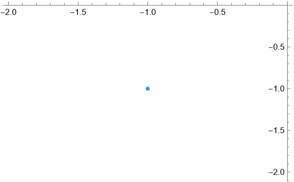
Remember that the angle we use for the Polar coordinates is from the positive x-axis and anticlockwise, so despite the angle in the ‘triangle’ between 45 degrees (picture it for yourself) the angle given to us in the Polar coordinates is π (135 degrees). Take note of that when using angles in other quadrants, and subtract the necessary amount (in this case, π radians). In this case r is , but when converting back into the Cartesian form we’d need to imagine the diagram above, and realise that both x and y coordinates are negative. Put simply, implies that x and y are positive, < θ ≤ π implies x is negative and y is positive, implies that x and y are negative, and < θ ≤ 2π implies y is negative and x is positive. Of course, note some overlap as a point lies on the axis (its up to you if you like to consider 0 positive). Some people prefer to let the angle be negative if the point is in the bottom two quadrants, but still measuring it from the positive x-axis: i.e. becomes -. I would personally recommend that you use the all-positive labelling.But that, put frankly, is all you need to know for simple Polar points. And there’s a handy function for plotting them too:
5
4
2
0≤θ≤
π
2
π
2
π<θ≤
3π
2
3π
2
3π
2
π
2
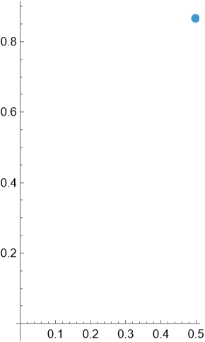
ListPolarPlot takes Polar coordinates in the form (θ, r), don’t let it worry you! Note this point is 1 unit from the origin.
In[]:=
ListPolarPlot[{{π/3,1}},PlotStyle->{PointSize[Large]}]
Out[]=
Lines and Circles in Polar Coordinates
Lines and Circles in Polar Coordinates
Some people find this topic quite hard to get their head around, especially when it can be easier to just convert back into Cartesian form. However, as said earlier, Polar coordinates can be very useful, and all of this is building up to that. If you think about it logically everything is very simple, but ensure that you don’t fall into the trap of thinking in Cartesian form, as it will prove problematic later on.
The first thing to think of is half-lines. These are lines that proceed in only one direction. We represent them using θ = a, where a is some constant angle. For example, if a is π we would see a line from the origin going to the left, in other words the x-axis only for negative x. These are very simple, so picture them in your mind - we’ll move on. Full lines can also be plotted. At this point we start using proper polar equations, which are of the form r = f(θ), where r is the distance from the origin as θ varies. For simple lines I will make you recall how we defined x and y in their polar forms - r*cos(θ), etcetera. Let’s think about that for a moment. r*cos(θ) = 2 is the same as saying x = 2. However, that’s not the form we like, so let’s divide by cos(θ). Once again, you may not have seen the reciprocal trig. functions - we abbreviate 1/cos(θ) as sec(θ), 1/sin(θ) as cosec(θ) and 1/tan(θ) as cot(θ). So our function becomes r = 2*sec(θ). We can plot this using the PolarPlot function of the Wolfram Language:
The first thing to think of is half-lines. These are lines that proceed in only one direction. We represent them using θ = a, where a is some constant angle. For example, if a is π we would see a line from the origin going to the left, in other words the x-axis only for negative x. These are very simple, so picture them in your mind - we’ll move on. Full lines can also be plotted. At this point we start using proper polar equations, which are of the form r = f(θ), where r is the distance from the origin as θ varies. For simple lines I will make you recall how we defined x and y in their polar forms - r*cos(θ), etcetera. Let’s think about that for a moment. r*cos(θ) = 2 is the same as saying x = 2. However, that’s not the form we like, so let’s divide by cos(θ). Once again, you may not have seen the reciprocal trig. functions - we abbreviate 1/cos(θ) as sec(θ), 1/sin(θ) as cosec(θ) and 1/tan(θ) as cot(θ). So our function becomes r = 2*sec(θ). We can plot this using the PolarPlot function of the Wolfram Language:
In[]:=
PolarPlot[2Sec[t],{t,0,2*Pi}]
Out[]=
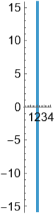
Note in the above I’ve let θ = t, for ease of use. The PolarPlot function assumes that our first argument is f(θ), and in the second argument we define what range that variable has. Remember that the line is infinite. You may also realise that we could easily make a horizontal line by using r = a*cosec(θ). These aren’t complicated lines, and we can also create other ones. These, and other graphs, may be harder to convert, but we only need to remember two things:- = + (by Pythagoras’ Theorem)- r*cos(θ) = x, r*sin(θ) = yThese allow us to convert to and from essentially any equations in Polar and Cartesian form. For example, let’s assume we have the line y = 2x - 5. Substituting our y and x for their counterparts gives r*sin(θ) = r*cos(θ) - 5. Rearranging gives r(sin(θ)-cos(θ)) = -5, which, remembering we want r alone, yields finally r = . It’s not very pretty, but it does the job:
2
r
2
x
2
y
-5
sin(θ)-cos(θ)
In[]:=
PolarPlot[-5/(Sin[t]-Cos[t]),{t,0,2*Pi}]
Out[]=
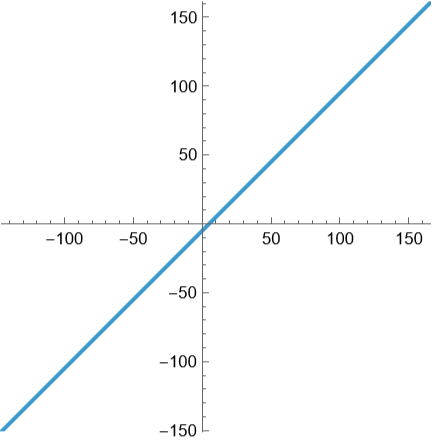
Which is perfectly correct.
As a last point, circles through the origin are very easy in Polar Coordinates - we just let r = a, where a is the radius, like so:
As a last point, circles through the origin are very easy in Polar Coordinates - we just let r = a, where a is the radius, like so:
In[]:=
PolarPlot[5,{t,0,2*Pi}]
Out[]=
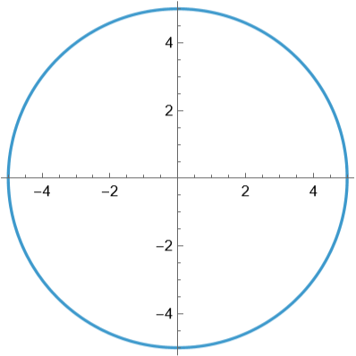
Note that in the Wolfram Language we should still specify that t is existent, even if we’re not using it.
We can also make some other neat circles very easily, for example r = a*sin(θ) is a circle with centre with it’s ‘base’ at the origin and height (diametre) a. We can convert more complicated circle formulae as we did earlier for lines.
We can also make some other neat circles very easily, for example r = a*sin(θ) is a circle with centre with it’s ‘base’ at the origin and height (diametre) a. We can convert more complicated circle formulae as we did earlier for lines.
More Complicated Graphs
More Complicated Graphs
This is where things start to get exciting. I’m not going to spend long here, because this is a ‘field’ (using the term loosely) that has endless possibilities. It’s where we see why Polar Coordinates are so important. Here’s an example:
In[]:=
PolarPlot[Sin[8*t],{t,0,2*Pi}]
Out[]=
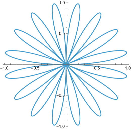
Not many realise that there can be flowers in maths, so take a moment to appreciate how brilliant it is that we can show one using one equation. If you try to think about converting it into Cartesian form things get very messy: we need sin(θ) not sin(8θ), so we end up using double angle formulae, complicating everything to a greater extent.
Some people restrict the values r can take to bigger than 0. If this happens, we would see a flower with only 8 petals. When we accept negative r values we end up with double that number, but only if the coefficient of θ in the sine function is even, for reasons I won’t go into. Here are some other graphs that are popular, and interesting:
Some people restrict the values r can take to bigger than 0. If this happens, we would see a flower with only 8 petals. When we accept negative r values we end up with double that number, but only if the coefficient of θ in the sine function is even, for reasons I won’t go into. Here are some other graphs that are popular, and interesting:
A Cardioid is represented by r = a*(p+q*cos(θ)), when p = q. When p is not equal to q we can describe it as a Limaçon, a family of curves which Cardioid is a member of.
Plots of form r = a + bθ plots are spirals; in specifying θ with a higher range (to 6 π) we see extra spirals added on.
All the graphs I have just shown you have some interesting theory behind them, which I will let you discover for yourself if you wish to. One thing I will tell you is that we can swap cosine for sine in all of the above, or vice-versa, which makes a very similar looking curve - perhaps you will realise why, as the two functions are translations of each other. They also all look particularly odd if you’re not used to Polar curves - we’d almost expect to see a piecewise function to define them, but that’s not the case.
The fact of the matter is that their Cartesian versions look very complicated, but in their Polar forms they’re very simple - and therefore easy to work with. For example, if we wanted the area of the graphs above it is far easier using the latter form. We’ll leave this topic here - I would highly recommend looking at other graphs, and practicing sketching them.
The fact of the matter is that their Cartesian versions look very complicated, but in their Polar forms they’re very simple - and therefore easy to work with. For example, if we wanted the area of the graphs above it is far easier using the latter form. We’ll leave this topic here - I would highly recommend looking at other graphs, and practicing sketching them.
3-Dimensional Polar Plots
3-Dimensional Polar Plots
Earlier I said how some people struggle with simple Polar functions like lines. 3-dimensional functions are therefore not to be considered until they have fully mastered the basics, because a great deal of visualisation is needed here for everything to make sense. At an introductory level, though, it can be much harder than this - just take care with how you’re picturing everything.
We can actually go into 3-dimensions in two ways: via Cylindrical Polar Coordinates, or Spherical Polar Coordinates, both of which we will consider briefly. A side note - unfortunately this isn’t as interesting as earlier, because everything gets exponentially more complicated when we want to portray nice-looking functions. This is all very important to know, however: and I personally enjoy the theoretical aspect of imagining the 3D world.
We can actually go into 3-dimensions in two ways: via Cylindrical Polar Coordinates, or Spherical Polar Coordinates, both of which we will consider briefly. A side note - unfortunately this isn’t as interesting as earlier, because everything gets exponentially more complicated when we want to portray nice-looking functions. This is all very important to know, however: and I personally enjoy the theoretical aspect of imagining the 3D world.
Cylindrical Polar Coordinates
Cylindrical Polar Coordinates
The reason for that is because Wolfram’s ‘official’ function for Cylindrical Polar plots doesn’t take coordinates, to my knowledge. That, for your reference, is RevolutionPlot3D, and can give some interesting 3D curves like so:
Spherical Polar Coordinates
Spherical Polar Coordinates
These are multiple spheres (consisting only of a surface), and shown like cross-sections so we can see them within each other.
Conclusion
Conclusion
That, more or less, is the fundamentals of Polar Coordinates. We’ve covered everything somewhat quickly, so if some of it has seemed confusing bear in mind that this sort of content would be covered over many lessons or lectures. Polar Coordinates are a vital part of mathematics, and are not to be underestimated - I highly recommend, once again, that you do your own research into them. Below I have given you the links of a couple of places that are good for further reading - the first especially so, if you want to consider calculus and other topics coming into play. I also hope you’ve realised how powerful a tool the Wolfram Language is for visualising Polar curves.
As always, I hope you found this useful! Until the next time.
As always, I hope you found this useful! Until the next time.
Further Reading
Further Reading
CITE THIS NOTEBOOK
CITE THIS NOTEBOOK
A beginner's guide to polar coordinates (with the Wolfram language)
by Leo Green
Wolfram Community, STAFF PICKS, January 18, 2026
https://community.wolfram.com/groups/-/m/t/3609057
by Leo Green
Wolfram Community, STAFF PICKS, January 18, 2026
https://community.wolfram.com/groups/-/m/t/3609057