HHL is a quantum algorithm that prepares a quantum state proportional to the solution of a linear system A x = b when A is Hermitian (or block-encodable as such) and b can be loaded as a state. You care about it when the goal is to estimate scalar functionals of the solution (overlaps or expectation values) rather than read out all coordinates, and when A admits efficient simulation so that the runtime can scale poly-logarithmically in the dimension under reasonable condition number and precision.
It works by loading the system register with the state encoding b, performing quantum phase estimation on a unitary generated by A to correlate each eigenstate with a digital phase label, using that label to drive a single-qubit rotation on a flag ancilla so its amplitude encodes the reciprocal of the estimated eigenvalue, uncomputing the label and reversing phase estimation, and finally post-selecting the flag. Conditioned on success, the system register is left in the direction of A⁻¹ b (normalized). You then measure task-specific observables on this state or compare it to a reference via overlaps. HHL is useful when you have efficient access to simulation of A, moderate condition number on the relevant subspace, and you only need compressed information about the solution; it is not a general replacement for classical solvers when you need the full vector or when A lacks a fast encoding.
It works by loading the system register with the state encoding b, performing quantum phase estimation on a unitary generated by A to correlate each eigenstate with a digital phase label, using that label to drive a single-qubit rotation on a flag ancilla so its amplitude encodes the reciprocal of the estimated eigenvalue, uncomputing the label and reversing phase estimation, and finally post-selecting the flag. Conditioned on success, the system register is left in the direction of A⁻¹ b (normalized). You then measure task-specific observables on this state or compare it to a reference via overlaps. HHL is useful when you have efficient access to simulation of A, moderate condition number on the relevant subspace, and you only need compressed information about the solution; it is not a general replacement for classical solvers when you need the full vector or when A lacks a fast encoding.
Install Wolfram quantum framework:
In[]:=
PacletInstall["https://www.wolfr.am/DevWQCF",ForceVersionInstall->True]<<Wolfram`QuantumFramework`
Out[]=
PacletObject

Generate a random Hermitian matrix :
A∈
n×n
In[]:=
n=4;a=QuantumOperator["RandomHermitian",n]["Matrix"]HermitianMatrixQ[a]
Out[]=
SparseArray

Out[]=
True
Generate a normalized random vector :
b∈
n
In[]:=
b=RandomVariate[CircularUnitaryMatrixDistribution[2^n]][[All,1]];Norm[b]
Out[]=
1.
Our main goal is to find that satisfies
x
A.x=b
Find the solution using classical linear solver and then normalize the result:
In[]:=
xClassical=LinearSolve[a,b]//Normalize
Out[]=
{-0.0310318+0.214092,-0.0814782+0.0908382,-0.20243+0.27246,-0.253612+0.292907,-0.152128+0.0721531,0.227304-0.223143,-0.29761-0.0905079,-0.0474046-0.0104791,-0.0721692+0.104622,-0.164166-0.332182,0.0292429+0.244291,0.316862+0.0640212,0.157334-0.0614232,0.17589-0.106518,0.187818-0.0698154,-0.119139+0.0204764}
Let’s find eigenvalues and eigenstates of :
A
In[]:=
{λ,u}=Eigensystem[a];u=Normalize/@u;λ=Chop@λ;
We will not use them for HHL, but only for some sanity check. In other words, is fed into HHL like a blackbox.
A
Choose such that the whole spectrum of lies in the principle internal
t
0
A
(-π/,π/]
t
0
t
0
In[]:=
t0=Floor@π/Norm[a](-π/t0<#<=π/t0)&/@λ//Apply[And]
Out[]=
1.50224
Out[]=
True
We shall take the Quantum-Phase-Estimation (QPE) unitary operator to be
U=
A
t
0
In[]:=
U=QuantumOperator[MatrixExp[t0Ia]];
U==
A
t
0
∑
j
λ
j
t
0
u
j
u
j
In[]:=
U["Matrix"]-MatrixExp[at0]//Chop//Flatten//DeleteDuplicatesU["Matrix"]-Exp[λt0].(KroneckerProduct[#,Conjugate[#]]&/@u)//Chop//Flatten//DeleteDuplicates
Out[]=
{0}
Out[]=
{0}
Set the number of phase-estimation qubits:
In[]:=
m=6;
Create circuits with the initial state
|〉|b〉
⊗m
0
In[]:=
stateprep=QuantumCircuitOperator[{QuantumState[b]}->m+Range[n]];
Create the Phase Estimation circuit for given :
U
m
In[]:=
qpe=QuantumCircuitOperator["PhaseEstimation"[U,m],Range[m+n]][[n+1;;-m-1]];
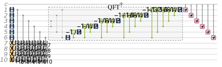
We have dropped some terms from the above circuit because our Phase Estimation circuit contains some NOT and measurement gates, too:
In[]:=
QuantumCircuitOperator["PhaseEstimation"[U,m],Range[m+n]]["Diagram"]
Out[]=
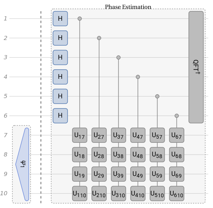
Put together the state and QPE in one circuit:
In[]:=
qc=QuantumCircuitOperator[{stateprep,"Barrier",qpe}];qc["Diagram"]
Out[]=
Given eigenvalues, find the corresponding single phase-estimate register that holds the eigenvalue estimate (i.e., the nearest lattice to the eigenvalue =Round):
*
y
j
m
2
t
0
λ
j
2π
In[]:=
yStar=ModRoundλ,
m
2
t0
2π
m
2
Out[]=
{33,34,29,28,26,39,39,24,45,18,17,51,53,8,60,1}
Given the initial state , write it in terms of normalized eigenstates of . It means
|b〉
U
|b〉=-1
n
2
∑
j=0
β
j
u
j
In[]:=
β=#.b&/@Conjugate[u];
The outcome of above circuit is state
qc|〉|b〉=-1-1|y〉≃-1
⊗m
0
n
2
∑
j=0
β
j
m
2
∑
y=0
1
m
2
1-Exp-y
t
0
m
2
λ
j
m
2
1-Exp-y
t
0
λ
j
m
2
u
j
n
2
∑
j=0
β
j
*
y
j
u
j
In[]:=
ψApproxQPE=β.MapThread[QuantumTensorProduct[QuantumState["Register"[m,#1]],QuantumState[#2]]&,{yStar,u}];ψExactQPE=Sumβ[[k]]QuantumTensorProductSumQuantumState["Register"[m,y]],{y,Range[0,-1]},QuantumState[u[[k]]],{k,Range@Length[u]};
1
m
2
1-Exp2πλ[[k]]-y
m
2
t0
2π
m
2
1-Exp2πλ[[k]]-y
t0
2π
m
2
m
2
Calculate the inner product of exact and approximated states vs the outcome of the quantum circuit:
In[]:=
Abs[ψApproxQPE["Dagger"][qc[]]["Scalar"]]^2Abs[ψExactQPE["Dagger"][qc[]]["Scalar"]]^2
Out[]=
0.30817
Out[]=
1.
Centered unwrapping of the nearest lattice to the eigenvalue =
:
y
j
|
In[]:=
yTilde=If[0<=#<=,#,#-]&/@Range[0,-1]
m-1
2
m
2
m
2
Out[]=
{0,1,2,3,4,5,6,7,8,9,10,11,12,13,14,15,16,17,18,19,20,21,22,23,24,25,26,27,28,29,30,31,32,-31,-30,-29,-28,-27,-26,-25,-24,-23,-22,-21,-20,-19,-18,-17,-16,-15,-14,-13,-12,-11,-10,-9,-8,-7,-6,-5,-4,-3,-2,-1}
Note the binary representation of the centered unwrapping of the nearest lattice to the eigenvalue is the same as the normal one (after some Mod ):
m
2
In[]:=
IntegerDigits[Mod[yTilde,],2,m]==IntegerDigits[Range[0,-1],2,m]
m
2
m
2
Out[]=
True
Given the centered unwrapping of the nearest lattice, compute the eigenvalue proxy =:
λ
y
2π
t
0
y
m
2
In[]:=
λTilde=
2π
t0
yTilde
m
2
Out[]=
{0.,0.0653522,0.130704,0.196057,0.261409,0.326761,0.392113,0.457465,0.522817,0.58817,0.653522,0.718874,0.784226,0.849578,0.91493,0.980283,1.04563,1.11099,1.17634,1.24169,1.30704,1.3724,1.43775,1.5031,1.56845,1.6338,1.69916,1.76451,1.82986,1.89521,1.96057,2.02592,2.09127,-2.02592,-1.96057,-1.89521,-1.82986,-1.76451,-1.69916,-1.6338,-1.56845,-1.5031,-1.43775,-1.3724,-1.30704,-1.24169,-1.17634,-1.11099,-1.04563,-0.980283,-0.91493,-0.849578,-0.784226,-0.718874,-0.653522,-0.58817,-0.522817,-0.457465,-0.392113,-0.326761,-0.261409,-0.196057,-0.130704,-0.0653522}
Create the corresponding eigenvalue-inversion circuit which is a collection of mutiplexers:
One can show that given the angles, the eigenvalue-inversion can be written as Gray-code circuit (which contains only 1 and 2 qubit gates):
Check the multiplexers and rotations are the same as Gray-code circuit:
Get the normalized final state of HHL circuit:
Find its amplitudes:
Compare the result with the one from the classical linear solver:
Harrow–Hassidim–Lloyd (HHL) algorithm as one function using Gray-code
Harrow–Hassidim–Lloyd (HHL) algorithm as one function using Gray-code
Create HHL circuit:
Given the result of above circuit, find corresponding amplitudes, and then normalize them to get solution of HHL solver:
Find the corresponding solution using classical approach:
Compare classical result with the quantum one (using the inner product as a measure; the closer to one the better)"
As mentioned, the number of phase-estimation qubits (3rd argument) determines the precision of final outcome. Execute HHL with less phase-estimation qubits::
Quantify the good ness of HHL result in compared with the classical result:
CITE THIS NOTEBOOK
CITE THIS NOTEBOOK
Harrow-Hassidim-Lloyd (HHL) algorithm: a step-by-step approach
by Mohammad Bahrami
Wolfram Community, STAFF PICKS, September 27, 2025
https://community.wolfram.com/groups/-/m/t/3552017
by Mohammad Bahrami
Wolfram Community, STAFF PICKS, September 27, 2025
https://community.wolfram.com/groups/-/m/t/3552017