CITE THIS NOTEBOOK: Mass-spring-damper, Romeo-Juliet, & Marital interaction models by Sangdon Lee. Wolfram Community OCT 27 2022.
CITE THIS NOTEBOOK: Mass-spring-damper, Romeo-Juliet, & Marital interaction models by Sangdon Lee. Wolfram Community OCT 27 2022.
Introduction
Introduction
I would like to introduce 3 models which seem very different but are equivalent in structure. What I mean by “equivalent or analogous structure” is the similarity among stock and flow variables and feedback loops. I will derive the MSD model in detail and discuss the similarity among the 3 models:
(1) mass-spring-damper model,
(2) Romeo and Juliet love affair model,
(3) marital Interaction model .
(1) mass-spring-damper model,
(2) Romeo and Juliet love affair model,
(3) marital Interaction model .
1
.Mass-spring-damper model
Mass-spring-damper (MSD) model is one of the most important models and this model is useful to understand other system such as electric circuits (see equivalent system in the appendix). The MSD model is also known as a damped harmonic oscillator.
https://en.wikipedia.org/wiki/Harmonic_oscillator
https://en.wikipedia.org/wiki/Harmonic_oscillator
x'[t]==v[t]
(
1
)v'[t]==-(c/m)*v[t]-(k/m)*x[t]
(
2
)2
.Romeo and Juliet love affair model
Dr. S.H. Strogatz wrote the first idea of how to model the love relationship between Romeo and Juliet and many updated models were published afterwords.
R'[t]=a*R[t]+b*J[t]
(
3
)J'[t]=c*R[t]+d*J[t]
(
4
)Strogatz, S. H. (1988) Love affairs and differential equations. Math. Magazine 61, 35.
A short introduction: http://educ.jmu.edu/~strawbem/Sample_Report.pdf
A short introduction: http://educ.jmu.edu/~strawbem/Sample_Report.pdf
3
.Marital interaction model
Dr. J. D. Murray who is a world well known expert in mathematical biology published a paper on modelling the dynamics of marital interaction. Their model is in difference equation form and very analogous to the Romeo and Juliet and MSD model . I don’t think Strogatz and Murray are aware of each other’s work.
W[t+1]==a+r1*W[t]+()
I
HW
H
t
(
5
)H[t+1]==a+r2*H[t]+()
I
WH
W
t
(
6
)Murray, J.D. (1993). Modelling the Dynamics of Marital Interaction: Divorce Prediction and Marriage Repair. In: Murray, J.D. (eds) Mathematical Biology. Interdisciplinary Applied Mathematics, vol 17. Springer, New York, NY. https://doi.org/10.1007/978-0-387-22437-4_ 5
John Gottman, Catherine Swanson, and James Murray, The mathematics of marital conflict: dynamic mathematical nonlinear modeling of newly wed marital interaction, Journal of Family psychology, 1999, v.13, no.1,3-19.
https://www.johngottman.net/wp-content/uploads/2011/05/The-Mathematics-of-Marital-Conflict-Dynamic-Mathematical-Nonlinear-Modeling-of-Newlywed-Marital-Interaction.pdf
Similar structure
Similar structure
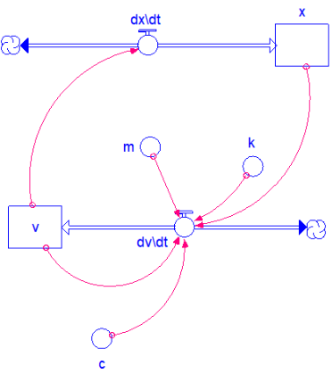
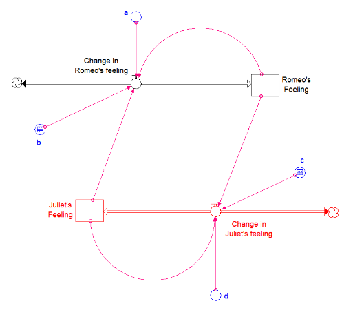
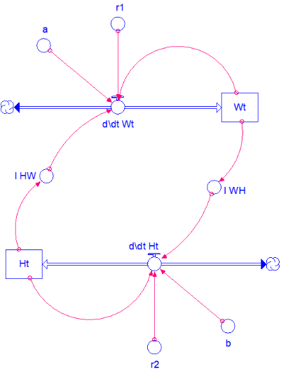
Three models are shown side-by-side, showing they are very analogous: mass-spring-damper system, Romeo and Juliet love affair model and marital Interaction model.
1. Mass-Spring-Damper model
1. Mass-Spring-Damper model
Description
Description
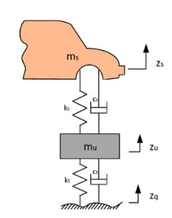
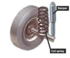
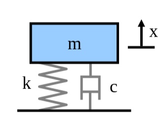
A good example of the MSD is to use the so called a quarter-car model as shown below. Only 1/4 of a car is analyzed (a car has 4 wheels/tires) and only vertical displacement is analyzed (a car moves in 3D space). I use displacement and distance interchangeably here but they are different concept. Displacement is a vector quantity having magnitude and direction (e.g., z-direction)
A quarter car schematic example is shown below:
⟹
Applying the Newton’s law
◼
F=m*a⟺=m*
∑
i
F
i
dV
t
dt
◼
Sum of forces = mass*acceleration
◼
n-th time-derivatives of position or displacement is as follows:
◼
position: x[t] ⇔ Velocity: v[t] ⇔Acceleration: a[t] ⇔ Jerk ⇔ Jounce (Snap) ⇔ Crackle ⇔ Pop
◼
x(t)⟹=v(t)⟹=a(t)=X(t)⟹Jerk,.....
∂X(t)
∂t
∂V(t)
∂t
2
∂
∂
2
t
◼
acceleration = time-derivative of velocity
◼
From empirical experiment, it is found that the spring force is proportional to displacement (aka. Hooke’s law)
◼
The direction of the restoring force from a spring is opposite to that of the displacement, so we have a negative sign.
◼
-k*
X
t
◼
dampingforceisproportionaltovelocity,,fromempiricalexperiment,
V
t
◼
-c*
V
t
◼
Puttingallforcestogether
◼
F=m*a⟺=m*⟺-c*-k*=m* ⟺-c*-k*=m*⟺m*+c*+k*=0 ⟺=-*-*X
∑
i
F
i
dV
t
dt
V
t
X
t
dV
t
dt
X
t
X
t
¨
X
t
¨
X
t
X
t
X
t
¨
X
c
m
X
k
m
Various ways of representing the same MSD model
◼
ODE form with one equation
◼
m*+c*+k*X=0
¨
X
X
◼
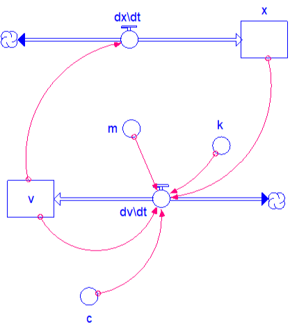
ODE form with two equations or state-space form
◼
dX
t
dt
V
t
◼
dV
t
dt
c
m
X
k
m
◼
Matrix form
◼
X t |
V t |
0 | 1 |
- k m | - c m |
x |
v |
X t |
V t |
Stock and Flow diagram
Stock and Flow diagram
dX
t
dt
V
t
dV
t
dt
c
m
Xt
k
m
Modeling
Modeling
Simulation
Simulation
Improvements
Improvements
◼
Simulate the following cases
◼
What if the car mass changes over time? The fuel of a car is consumed so the car mass changes
◼
What if the spring force is non-linear such as a broken spring?
◼
What if the damping force is non-linear such as a leaking damper
◼
More importantly, demonstrate a resonance frequency
◼
Add a sinusoidal forcing function (e.g., amplitude*Sin[2*Pi*frequency*t] ) to this model, change the frequency and identify the resonance frequency that will make the displacement fluctuate a lot. A car travels on uneven or rough road which puts a force to a car body. At a certain frequency, the force from the road will make the car body vibrates violently, this frequency is called resonance frequency. For example, we can find a You tube clip showing that a Ford F-150 shakes dangerously once it is driven at certain speed.
2. Romeo and Juliet love affair model
2. Romeo and Juliet love affair model
Description and interpretation of the differential equations
Description and interpretation of the differential equations
Note that the parameters (a,b,c,d) are dimensionless fraction and can be better understood if they are changed to 1/Time_To_Adjutments. For example, “a”=0.25= 1/TimeToAdjus, meaning it takes about 4 month for the Romeo's feeling rise to 63 % of the step input of 100. Therefore the parameters indicate time delay!
Notice that the “a*R[t]" and “d*J[t]" are analogous to the damping force in MSD model. They represent a situation where hot or cold feeling dissipate over time
Stock and flow diagram
Stock and flow diagram
Modeling
Modeling
Differential equation
Differential equation
Simulation
Simulation
Improvements
Improvements
◼
Simulate the following cases
◼
Romeo and Juliet fall in love at the first sight
◼
Romeo likes Juliet but she does not like him
◼
Romeo likes Juliet but she is indifferent to him.
◼
Romeo and Juliet fall in love at the first sight and their feeling becomes neutral, not hot nor cold, like a long-time best friend.
◼
More importantly, introduce an ex-boyfriend or ex-girl friend who has the same stock-flow structure. The ex-boyfriend and ex-girlfriend may and may not know with each other. I developed this model and this addition will make the system behave very complicated.
3. Marital Interaction model
3. Marital Interaction model
◼
H[t] is for husband’s emotion and W[t] is for wife’s emotion
◼
“a” and “b” are to represent the general characters of a husband a wife, whether they are positive or negative generally.
◼
Model
Appendix
Eigenvalue and eigenvectors of MDS model
Eigenvalue and eigenvectors of MDS model
Symbolic solution of the MSD model
Symbolic solution of the MSD model
Eigenvalue and Eigenvector of MSD model
Eigenvalue and Eigenvector of MSD model
◼
The real parts of eigenvalues are all negative, so this mass-spring-damper system is stable!
Equivalent system
Equivalent system
Many systems are equivalent even though they look different. For example, the charge in electrical system is analogous to the position (x[t]) and current is analogous to velocity. Notice that at the last row shows the various differential equations but they are equivalent.
Stock and flow are a fundamental concept
Stock and flow are a fundamental concept
◼
The stock and flow is a fundamental concept .
◼
The x[t] is known as a stock variable (or state variable in calculus) and shown as a rectangular box in System Dynamics . The x[t]/t is known as a flow variable (or derivative) and shown as a pipe with one or two arrows at the end. The stock- flow diagram is analogous to the bathtub in a house . Water flows into a bathtub and flows out via a drain (inflow and outflow) . If inflow > outflow, then the water in the bathtub will increase, and vice versa.
◼
Confusing stocks with flows makes it difficult to understand the cause and effect relationship to improve a system. For example, one confusion is the belief that when inflow decreases then stock decreases and vice versa and we expect a positive correlation.
◼
Reducing CO2 “emission” will not reduce the CO2 in the atmosphere unless the CO2 emission is lower than the CO2 absorption, which is very disturbing.
◼
For example, reducing "CO2 emission" (an inflow) does not decrease "CO2 in the atmosphere" (a stock) unless the CO2 emission is lower than the CO2 absorption. The "CO2 in the atmosphere" continues to increase at a slower rate. This could be understood using the following analogy. if someone is driving on a high way at the speed of 100 kph and had to reduce the speed to 50 kph due to construction, he or she still drove “more” distance but not as much as 100 kph. The traveled distance continue to increase but at a slower rate.
◼
The CO2 increases considerably after 1950 especially. What this means is that the ” CO2 emission” must be lower than the CO2 emission in 1950 (assuming that the atmospheric CO2 level must be reduced to the 1950 level, about 300 ppm ) because we already pumped a lot of CO2 into the atmosphere. The only way to reduce the “atmospheric” CO2 is to make that the CO2 emission (inflow) be much lower than the CO2 absorption (outflow), that is the CO2 emission must be below the 1950 level, about 5 billion tone.
◼
The char in the right is the CO2 in the atmosphere (stock) and the chart in the left is the CO2 emission (flow)
◼
Reducing CO2 emission will not reduce the CO2 in the atmosphere unless the CO2 emission is lower than the CO2 absorption