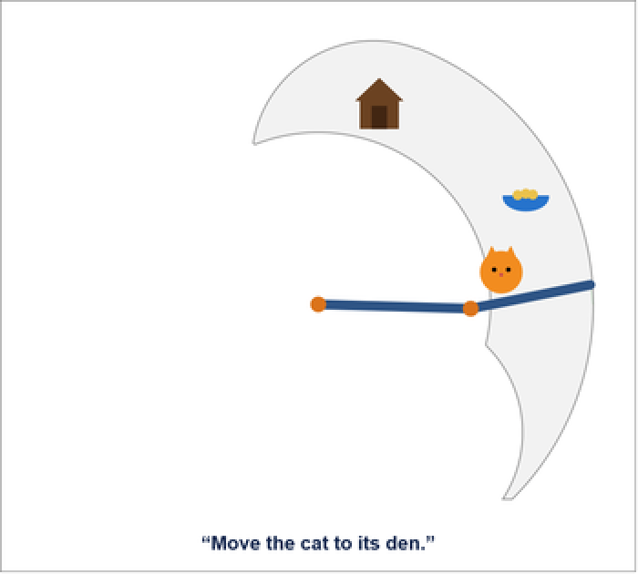
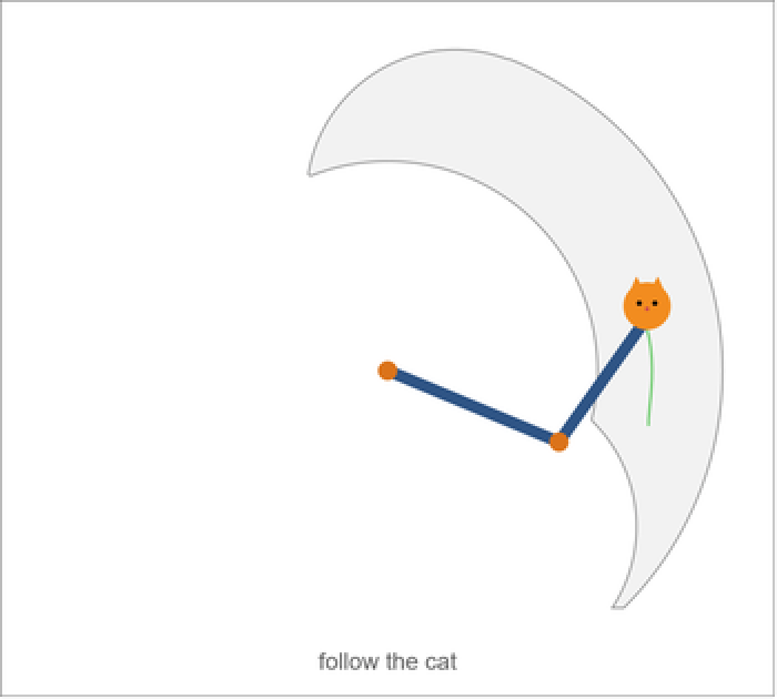
This notebook builds a robot arm that acts on its own. It looks at a scene, understands a plain-English request, and carries it out. I built this with Wolfram System Modeler and the Wolfram Language, starting from a standard robot-description file and ending with an arm that sees, reasons, and moves.
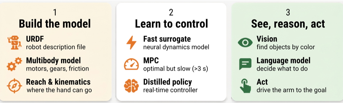
The work has three parts:
1. Build the model: Turn a robot description into a physical model with motors and friction, and find where the arm can reach.
2. Learn to control\b: Train a fast neural surrogate of the arm’s dynamics, use it for model-predictive control, learn a real-time policy from it.
3. See, reason, act: Find objects with image processing, let a language model decide what to do, and drive the arm to complete the task.
2. Learn to control\b: Train a fast neural surrogate of the arm’s dynamics, use it for model-predictive control, learn a real-time policy from it.
3. See, reason, act: Find objects with image processing, let a language model decide what to do, and drive the arm to complete the task.
Step 1—How do we model and simulate the arm?
Step 1—How do we model and simulate the arm?
To control an arm, we first need a high-fidelity model of it that behaves like the real thing. So the first task is to turn a robot description into a physical model and add additional dynamics like electric motor actuators, gears and damping.
Robots are usually described by a URDF file. This is an XML file that lists the arm’s links (their mass, size, and inertia) and its joints (their axis of rotation and motion limits). We use a SCARA-style robot: a shoulder joint and an elbow joint, both turning about a vertical axis, with a heavier first link and a lighter second link. I used the SCARA arm as it works in a horizontal plane, and keeps the example easy to follow.
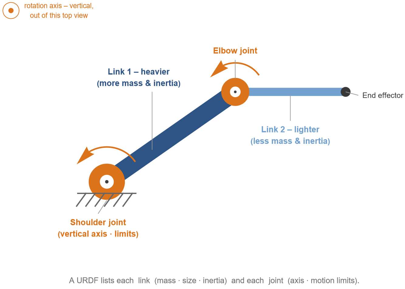
Here is the URDF description. I have shown it only for reference, so you can see what information a URDF carries. Each link declares a mass and a box geometry, and each joint declares an axis and angle limits.
urdf = "<robot name='scara2'>
<link name='base'/>
<joint name='shoulder' type='revolute'>
<parent link='base'/><child link='link1'/>
<origin xyz='0 0 0'/>
<axis xyz='0 0 1'/><limit lower='-1.0' upper='1.2' effort='50' velocity='3'/>
</joint>
<link name='link1'>
<inertial><origin xyz='0.125 0 0'/><mass value='3.08'/></inertial>
<visual><origin xyz='0.125 0 0'/><geometry><box size='0.25 0.04 0.04'/></geometry></visual>
</link>
<joint name='elbow' type='revolute'>
<parent link='link1'/><child link='link2'/>
<origin xyz='0.25 0 0'/>
<axis xyz='0 0 1'/><limit lower='-1.8' upper='1.8' effort='20' velocity='5'/>
</joint>
<link name='link2'>
<inertial><origin xyz='0.10 0 0'/><mass value='1.39'/></inertial>
<visual><origin xyz='0.10 0 0'/><geometry><box size='0.20 0.03 0.03'/></geometry></visual>
</link>
</robot>";
<link name='base'/>
<joint name='shoulder' type='revolute'>
<parent link='base'/><child link='link1'/>
<origin xyz='0 0 0'/>
<axis xyz='0 0 1'/><limit lower='-1.0' upper='1.2' effort='50' velocity='3'/>
</joint>
<link name='link1'>
<inertial><origin xyz='0.125 0 0'/><mass value='3.08'/></inertial>
<visual><origin xyz='0.125 0 0'/><geometry><box size='0.25 0.04 0.04'/></geometry></visual>
</link>
<joint name='elbow' type='revolute'>
<parent link='link1'/><child link='link2'/>
<origin xyz='0.25 0 0'/>
<axis xyz='0 0 1'/><limit lower='-1.8' upper='1.8' effort='20' velocity='5'/>
</joint>
<link name='link2'>
<inertial><origin xyz='0.10 0 0'/><mass value='1.39'/></inertial>
<visual><origin xyz='0.10 0 0'/><geometry><box size='0.20 0.03 0.03'/></geometry></visual>
</link>
</robot>";
Each piece of the URDF maps directly onto a System Modeler (Modelica) component, so building the model is mostly a translation exercise.
A <link> becomes a BodyBox (Modelica.Mechanics.MultiBody.Parts.BodyBox), a rigid box whose mass and inertia are computed from its dimensions (r, width, height) and density (default 7700, steel). In the model we have, for example, bodyBox1(r = {0.25, 0, 0}, width = 0.04, height = 0.04).
A revolute <joint> becomes a Revolute joint (Modelica.Mechanics.MultiBody.Joints.Revolute). Its axis parameter n sets the direction of rotation, a unit vector fixed in frame_a with default {0, 0, 1}.
Add the actuators
Add the actuators
A description of links and joints captures the arm’s geometry, but a real arm also has actuators. Without them it cannot move, and our control signal would have nowhere to go. So at each joint we add a voltage-driven DC motor, a gearbox, and bearing friction. This makes our control input a real physical quantity, a voltage, and it lets the learned controller transfer to something realistic later.
In[]:=
Import[FileNameJoin[{NotebookDirectory[],"ScaraArm.mo"}],"MO"];scara=SystemModel["ScaraArm"];SystemModel[scara,{"Diagram",Frame->False,ImageSize->Large}]
Out[]=
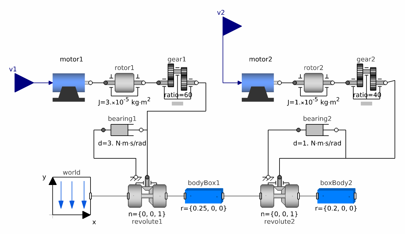
Two details are worth knowing. The shoulder uses a bigger motor with a higher gear reduction than the elbow and carries the heavier link, so the two joints respond very differently to the same command. And because a SCARA works in the horizontal plane, gravity points straight down through the joint axes and produces no joint torque.
Simulate and check the behaviour
Simulate and check the behaviour
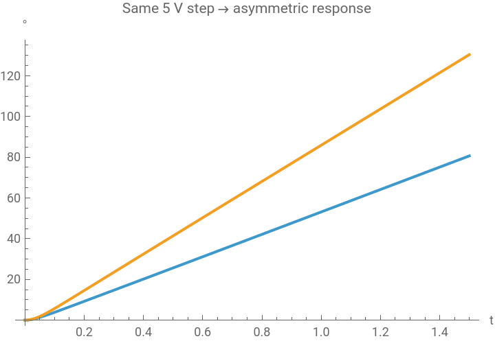
We apply a 5-volt step to both motors and plot the two joint angles over time. The elbow has a smaller, faster motor and a lighter link, so it should accelerate faster than the heavier shoulder.
chk=SystemModelSimulate[scara,{0,1.5},<|"Inputs"->{"v1"->(5.&),"v2"->(5.&)}|>];SystemModelPlotchk,{"revolute1.phi","revolute2.phi"},
Out[]=


Step 2—Where can the arm reach?
Step 2—Where can the arm reach?
To give the arm goals, points to move to, we need two things.
First, a way to turn joint angles into a hand position (end effector’s position), the forward kinematics. Second, a map of which hand positions are reachable, the workspace. Without the first, we cannot relate motor commands to where the hand ends up. Without the second, we might ask the arm to reach somewhere it physically cannot, then wrongly blame the controller.
Forward kinematics: Derived automatically from the System Modeler (Modelica) model
Forward kinematics: Derived automatically from the System Modeler (Modelica) model
The forward kinematics is the formula giving the end effector’s (x, y) position from the two joint angles. Rather than deriving it by hand, we read it straight out of the compiled model, so the formula is guaranteed to match the simulation exactly. The helper package adjointFromJSON.m queries System Modeler’s internal equations and returns a closed-form expression for any variable in the model.
We load the package and parse the model. parseBlockdebug simulates the model once and extracts its full equation structure. listStates lists the variables the solver treats as the system’s state.
In[]:=
Get[FileNameJoin[{NotebookDirectory[],"adjointFromJSON.m"}]];parsed=parseBlockdebug["ScaraArm"];listStates[parsed]
Out[]=
{bearing2.phi_rel,bearing2.w_rel,bearing1.phi_rel,bearing1.w_rel,motor1.inductor.i,motor2.inductor.i}
Six states come back: the two joint angles and their speeds, plus a current inside each motor. The motors’ electrical dynamics are much faster than the arm’s motion, so for control we keep just the four mechanical states. (The angle is carried by the bearing, hence the bearing.phi_rel names. I will show later that it is identical to revolute.phi.)
Now we read the closed-form expression for the end effector's x- and y-coordinate directly from the model and wrap it as a function fkS of the two joint angles.
In[]:=
phiA=Symbol[mangleName["bearing1.phi_rel"]];phiB=Symbol[mangleName["bearing2.phi_rel"]];fkExprs=Quiet@Simplify[equationFor[parsed,"boxBody2.frame_b.r_0["<>ToString[#]<>"]"]["Expression"]]&/@{1,2};fkS[{p1_,p2_}]:=fkExprs/.{phiA->p1,phiB->p2};
clean[expr_]:=expr//Rationalize//Simplify//TrigReduce//prettify;FramedGrid[{{"x","=",clean[fkExprs[[1]]]},{"y","=",clean[fkExprs[[2]]]}},Alignment->{{Right,Center,Left},Baseline},Spacings->{0.7,1.4}],
Out[]=
The result is the familiar two-link forward kinematics: x = 0.25 cos(phi1) + 0.20 cos(phi1 + phi2), and similarly for y. We never had to derive it. It came directly from the equations the System Modeler uses.
Aside: are the bearing and revolute angles the same?
Aside: are the bearing and revolute angles the same?
You may have noticed the extracted kinematics use bearing1.phi_rel, while we named the joint revolute1.phi. Before trusting the formula, it is worth confirming these are the same physical angle. Otherwise our targets and our control would live in different coordinate systems. Because the bearing sits directly across the joint, the two are the same angle. The compiler keeps one of them and records the rest as aliases. We can prove it with a one-hop graph query.
A single-hop path confirms it: revolute1.phi and bearing1.phi_rel are interchangeable, so the controller can read either.
The reachable workspace
The reachable workspace
Finally we answer the question: where can the hand actually go?
Knowing this lets us place only achievable targets later, and recognise when a request is impossible rather than blaming the controller. Because we already have the closed-form kinematics, we do not need a simulation per pose. We sample many joint-angle pairs across their limits and evaluate fkS on each. The left plot shows the sampled joint angles. The right shows the resulting hand positions, the arm’s reachable workspace, a curved patch whose shape is set by the link lengths and the joint limits.
Step 3—How do we build a fast model of the arm?
Step 3—How do we build a fast model of the arm?
We could compute the joint angles that put the hand on a target with inverse kinematics, then drive there with a simple joint controller. But that ignores the arm’s dynamics, its inertia, its motors, and its limits, and tends to be jerky and imprecise. A better controller plans using a model of how the arm responds to voltages, and re-plans as it moves. The problem is that the full multibody model is far too slow to evaluate inside a real-time control loop. So in this step we train a lightweight neural network to imitate it: a surrogate that predicts, in one quick evaluation, how the arm responds to a given voltage.
The controller we are heading toward issues a new voltage every 0.1 seconds and holds it steady in between, so we generate training data the same way. We drive each joint with a random voltage that changes every 0.1 seconds, and record the state at each instant. The helper mkPC turns a list of voltage levels into a piecewise-constant signal. encC packages a state and voltage into the network’s input, feeding each angle as its cosine and sine, which avoids the discontinuity when an angle wraps past plus or minus pi.
It helps to see what that control signal looks like. Each level is held flat for one 0.1-second interval (a zero-order hold), clipped to plus or minus 10 V.
Using the parsed model, we pick out the four mechanical states, the two joint angles and their speeds, and order them shoulder-first. This sState is what the surrogate predicts and what the controller reads.
Generate training data
Generate training data
A surrogate is only as good as the data it sees, so we want examples that span the arm’s whole working range. We run 40 short simulations, each starting from a random pose and joint speed and driven by fresh random voltages, and record the data as pairs. From the current state and applied voltage, what is the change in state over the next 0.1 seconds? Predicting the small change is easier and more accurate to learn.
A quick look at the training set: the eight inputs (the two angles as cos/sin pairs, the two speeds, and the two voltages) and the four outputs (the one-step change in each state). The outputs cluster tightly around zero, since each step is a small change.
Standardize and train
Standardize and train
The raw inputs live on very different scales. Cosines and sines sit in [-1, 1], while voltages reach plus or minus 10. A network trained on those would pay outsized attention to the large-valued features. So we standardize every input and output to mean 0 and standard deviation 1, putting them on equal footing, then train a small network to map standardized inputs to standardized outputs. The wrapper stepC applies the trained network to advance the arm’s state by one 0.1-second step. This is our fast stand-in for the full simulation.
Does the surrogate match the simulator?
Does the surrogate match the simulator?
Before trusting the surrogate inside a controller, we check it against the real thing. We drive both the true model and the surrogate from the same state with the same voltages and overlay the resulting trajectories. The surrogate is a one-step predictor used over many steps, so small errors accumulate. What we are really checking is that it tracks well over the short horizon the controller uses.
Step 4—How do we control the arm?
Step 4—How do we control the arm?
With a fast model in hand, we can control the arm. Model-predictive control (MPC) is a natural fit. At each instant it asks which short sequence of voltages best drives the hand to the target and brings it to a stop. It answers by simulating every candidate through the surrogate, applies only the first voltage of the winner, then re-plans from the new state. Re-planning every step is what lets it reach any target and correct its own mistakes along the way.
We build it in three pieces. mpcRoll rolls the surrogate forward under a candidate voltage sequence. costT scores a sequence, heavily for ending on the target, with smaller penalties for still moving, for straying on the way, and for using large voltages. mpcAct searches for the best first voltage to apply right now. reachMPC closes the loop, re-planning at every step.
Let us send the hand to a test point and confirm it arrives.
How fast is it?
How fast is it?
MPC was able to make the hand reach its target, but there is a cost we have to measure, because it decides whether this controller can run on a real arm at all. We time each control decision.
Each decision takes about 3 seconds, but the controller is meant to issue a new voltage every 0.1 seconds. This optimizer is roughly 30 times too slow to run in real time. It would still be planning its next move long after the arm needed to make it. That makes MPC a great teacher but a poor real-time controller, so we use it offline. In the next step we let this slow optimizer generate a library of expert demonstrations, then distill them into a network that maps state and target straight to a voltage in a single, sub-millisecond evaluation. The optimization happens once, in advance. What runs on the arm is fast enough to close the loop.
Step 5—How do we control the arm fast?
Step 5—How do we control the arm fast?
Generate demonstrations
Generate demonstrations
The plan is to amortize the optimizer. We run the slow MPC offline across many starting states and targets, record the voltage it chose in each, and train a network to reproduce those choices. This section produces the training set, and it is the one slow step, a few minutes here and possibly hours for a complex model, because it runs the optimizer hundreds of times. It only needs to run once.
Because the target can change at run time, we do not bake in a single goal. Each demonstration pairs a random starting state with a random reachable target. costT scores a candidate voltage sequence for a given (state, target) pair. solveDemo runs the optimizer once from that state and returns just the optimal first voltage.
First, a few geometry helpers: forward kinematics (fkA), inverse kinematics (ikS), the arm’s link points for drawing (armPts), and reachQ, which tests whether a target lies inside the arm’s reachable workspace given its joint limits.
We sample 500 demonstrations. Most start from a random state with a random reachable target, spread broadly so the policy sees the whole task. The rest start near their own target’s goal pose, so the controller also demonstrates how to slow down and stop, at whatever target it is given rather than one fixed point.
Solving 500 MPC problems is slow, so we run it once in parallel and cache the result to demos.mx. Set recompute to False afterwards to reload instead of re-solving (and back to True whenever the demonstrations change).
Distill the policy
Distill the policy
Now we distill those demonstrations into a network that maps the current state and the desired target to the two motor voltages the controller would have chosen. There is no optimization in the loop, just one fast evaluation per step. Because the target varies across the demonstrations, the policy generalizes to targets chosen on the fly rather than memorizing one. As with the surrogate, we standardize the inputs so every feature carries comparable weight. The target coordinates are small next to the cos/sin features and would otherwise be under-weighted.
How well does it work, and where?
How well does it work, and where?
A single successful reach is not enough evidence. We want the policy’s accuracy across the whole workspace. We sweep targets over the reachable region, run the policy to each from rest, and colour by the final distance to the target. We evaluate only inside the reachable boundary.
The error stays around a centimetre across the reachable workspace, and the network evaluates in well under a millisecond, about a thousand times faster than the MPC it learned from. The slow optimum, computed once, now runs in real time.
Moving target
Moving target
The heatmap showed the policy is accurate. Accuracy is only half of what distillation bought us. The other half is speed. The MPC teacher needed about three seconds per decision. The distilled policy answers in well under a millisecond. The clearest way to see what that unlocks is to give it a target that moves. The slow MPC could never follow one, since it would still be planning while the target slid away. The real-time policy keeps pace, trailing by only a small, steady lag.
The lag comes from how the policy was trained. It learned to reach a target, so it always aims where the target is now and arrives a beat later. The faster the target moves, the bigger the lag. We can show this directly by sweeping the target speed.
And here it is in motion, the arm chasing the moving target in real time.
Static reaches showed the policy is accurate to about a centimetre. This moving-target test shows it is fast enough to track in real time. The distilled policy is both accurate and fast.
Step 6—How does the arm see the scene?
Step 6—How does the arm see the scene?
So far the arm reaches coordinates we hand it. To act in the real world it has to find them itself, by looking. So we give it eyes: a camera image of its workspace holding a few objects, a cat to move and two places it might go (its den and its food bowl). We locate each object by colour. We keep the pixels close to that colour, then take the centre of the largest blob. Then we convert pixel locations into workspace coordinates.
First the detection and calibration helpers. detect finds the largest blob of a given colour. detectWorld converts its pixel centre into world coordinates, reading each image’s own dimensions so the same code works for a synthetic frame, a photo, or a live camera. toScene is the inverse map, used only to place the icons when we draw the scene.
Now the objects themselves, drawn as simple coloured icons: a cat (orange), a den (brown), and a food bowl (blue). Each has one dominant colour, which is all the detector needs.
We render the scene, then detect each object by its colour and confirm all three lie within the arm's reach.
Step 7—How does the arm reason about a request?
Step 7—How does the arm reason about a request?
Vision tells the arm where things are, but not what to do with them. Interpreting a plain-English instruction into an ordered plan is what a language model is good at. We give an LLM the object names and the instruction, and ask for the order in which to visit them. The vision system supplies the coordinates. The language model decides what to do. With several objects in the scene, the same arm follows whatever the sentence asks: “move the cat to the den”, or “take the cat to its food”.
SpeechRecognize turns a microphone recording into text, which we hand to the same planner, so the whole task can begin from a sentence said out loud. (You can test it without a microphone using SpeechRecognize[SpeechSynthesize[“...”]].)
In[]:=
instruction = SpeechRecognize[spoken];
plan = ToExpression@planner[ToString[Keys[scene]], instruction]
plan = ToExpression@planner[ToString[Keys[scene]], instruction]
Complete the task
Complete the task
Everything comes together here. We turn the plan into a sequence of targets, drive the hand to the first named object with the controller, then carry it to each remaining destination. The cat rides along with the hand, so it reads as a pick-and-place even though the arm has no gripper. The result is a task posed as a sentence, grounded by vision, ordered by a language model, and executed by the controller we built from scratch.
Putting it all together—a voice-controlled arm
Putting it all together—a voice-controlled arm
Finally, we wrap the whole pipeline. Press Record and speak a command, “move the cat to the den” or “take the cat to its food”, and the panel transcribes your words, shows them on screen, asks the language model for a plan, and animates the arm carrying it out. Vision finds where, the language model decides what, the policy works out how, and you only had to say a sentence. A text field is included as a fallback, so it works even without a microphone.
Putting it all together—tracking a moving cat
Putting it all together—tracking a moving cat
One last test. Everything so far reached static targets, but the cat doesn’t sit still, so we let it wander and ask the arm to follow. This is something the original MPC controller could not do: at about 3 seconds per decision it would still be planning while the cat strolled away. The distilled policy decides in well under a millisecond, so it tracks the moving cat in real time, trailing by only a small, steady lag.
Summary
Summary
We started with a URDF and finished with an arm that sees, reasons, and acts. Along the way we built a physically faithful, voltage-driven model; mapped its reach; trained a fast surrogate of its dynamics; designed an optimizing controller and distilled it into a real-time policy; and added vision and language so a task could be given as simply as a photo and a spoken sentence.
Each layer uses a distinct topic: multibody modeling, optimization, machine learning, image processing, and large language models.
Three ideas carried the whole project. Get the model right first: realistic motors and damping made the arm both believable and learnable, where an idealized model would neither control nor transfer well. Amortize the optimizer: running the slow optimal controller offline and learning from it turns it into a fast, real-time one. And let each tool do its job: vision provides where, the language model decides what, and the controller works out how.
CITE THIS NOTEBOOK
CITE THIS NOTEBOOK
Building a self-driving robot arm: from a URDF to vision-and-language control
by Ankit Naik
Wolfram Community, STAFF PICKS, June 26, 2026
https://community.wolfram.com/groups/-/m/t/3739835
by Ankit Naik
Wolfram Community, STAFF PICKS, June 26, 2026
https://community.wolfram.com/groups/-/m/t/3739835