Logistic Growth
Logistic Growth
Logistic growth is defined by a differential equation.
f(t)/t==k f(t) (1-f(t)/L) ,
where k is a continuous growth rate and L is the limit to growth such that f(t) cannot exceed L. When f(t) is small relative to L, (1-f(t)/L) is near 1. Then the initial growth is proportional to f(t) with exponential growth rate, k. When f(t) reaches L growth rate is zero and growth stops. If we require that L and k be positive, then the growth rate is always positive.
The model was originally developed to account for population growth, with the idea that there was a maximum population, L, that a space could support, and population could not grow beyond that maximum in the space. With epidemiologic control of an infection, there is a similar model, which is to confine the infected and exposed population so that the members cannot spread the infection to the much larger general population. This can take a while to accomplish at the beginning of an outbreak, because the exposed population isn't well known. But the main idea is to confine infected people and people at risk to a segregated population space, where L is much smaller than it would be for the population at large. It is also important that the contacts be isolated from each other. The idea here is that if the control is good, the virus has a limited population to which it can spread. Susceptibility levels don't matter if the infection cannot reach the whole population. If the isolation is not done carefully, there is some risk of increased infection in the confined space, say a cruise ship where no passengers are let off the ship.
More information and history.
DSolve[{f'[t]==kf[t](1-f[t]/L),f[t0]==L/2},f[t],t]//FullSimplify
Out[]=
f[t]L+
kt
kt
kt0
This can be simplified
FullSimplifyL+==L(1+E^(-k(t-t0)))
kt
kt
kt0
Out[]=
True
In[]:=
logisticGrowth[t_,{t0_,k_,L_}]:=L/(1+E^(-k(t-t0)));
This proves the differential equation solution.
D[logisticGrowth[t,{t0,k,L}],t]==klogisticGrowth[t,{t0,k,L}](1-logisticGrowth[t,{t0,k,L}]/L)//FullSimplify
Out[]=
True
The boundary condition, f(t0) == L/2, sets t0 to be the inflection point where growth rate is maximum.
Solve[D[logisticGrowth[t,{t0,k,L}],{t,2}]==0,t,Reals]
Out[]=
{{tt0}}
The function gives a sigmoid curve and the first derivative is also shown.
Plot[{logisticGrowth[t,{20,0.2,100}],Evaluate@D[logisticGrowth[t,{20,0.2,100}],t]},{t,1,40},GridLinesAutomatic,PlotRangeAll]
Out[]=
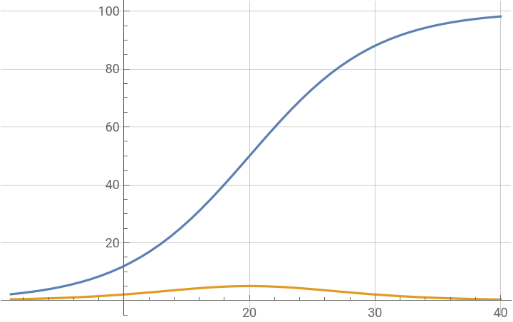
With parameter substitution, the logistic growth function becomes the LogisticDistribution function.
logisticGrowth[x,{μ,1/σ,1}]CDF[LogisticDistribution[μ,σ],x]
Out[]=
1
1+
-
x-μ
σ
Out[]=
1
1+
-
x-μ
σ
Data Source
Data Source
In[]:=
confirmed=Import["https://raw.githubusercontent.com/CSSEGISandData/COVID-19/master/csse_covid_19_data/csse_covid_19_time_series/time_series_19-covid-Confirmed.csv"];confirmed[[1]][[-1]]
Out[]=
2/24/20
In[]:=
deaths=Import["https://raw.githubusercontent.com/CSSEGISandData/COVID-19/master/csse_covid_19_data/csse_covid_19_time_series/time_series_19-covid-Deaths.csv"];deaths[[1]][[-1]]
Out[]=
2/24/20
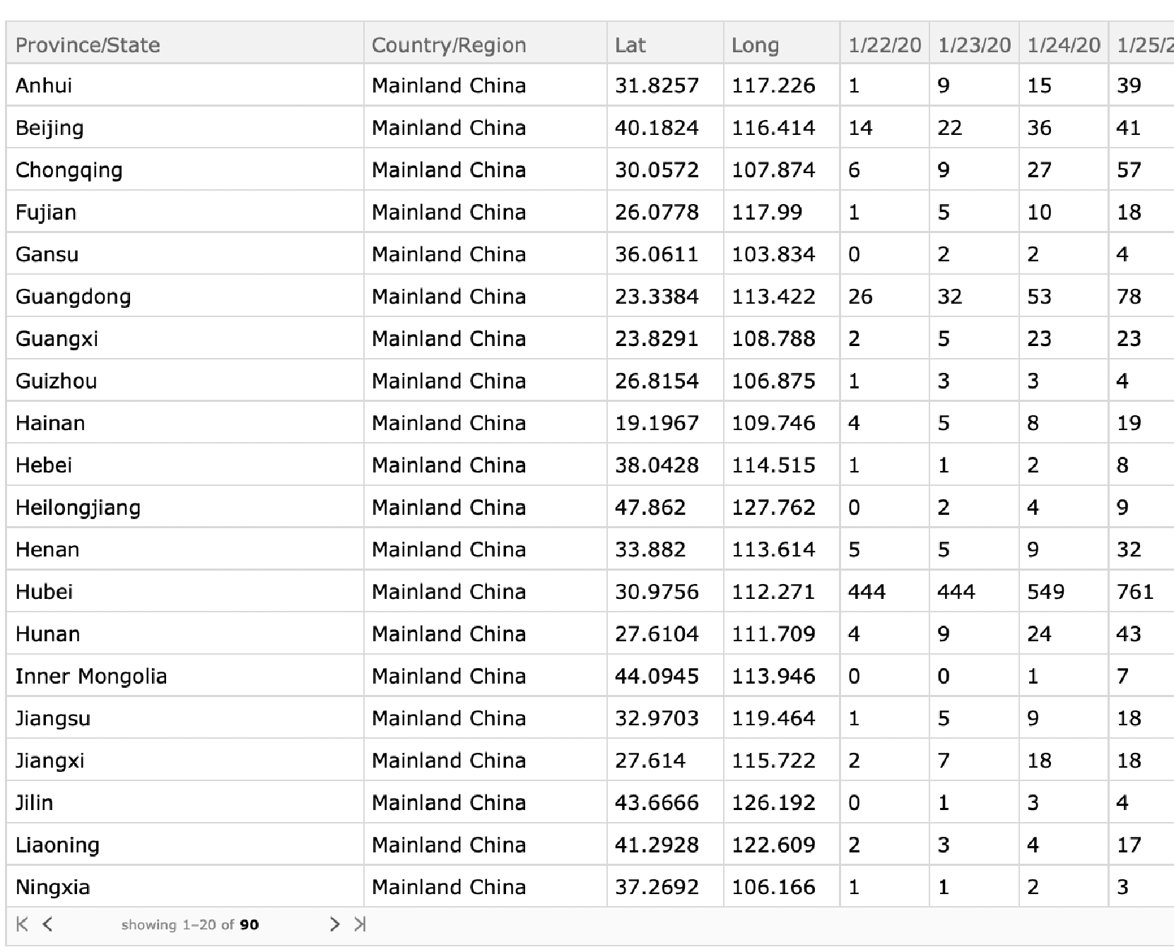
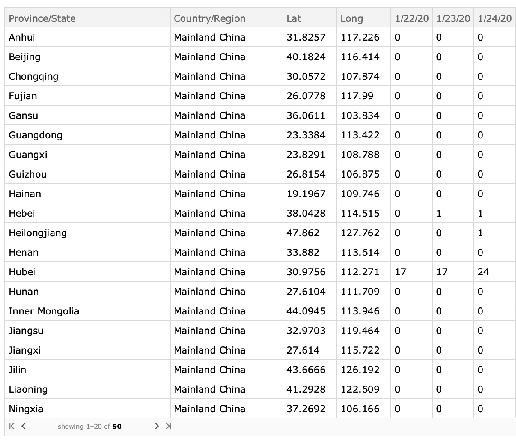
The data are also available as ResourceData["Epidemic Data for Novel Coronavirus COVID-19"]; The GitHub data appears to be the same. For the model the GitHub data are in a simpler format.
confirmedData=AssociationThread[First@confirmed,#]&/@Rest[confirmed]//Dataset
deathData=AssociationThread[First@deaths,#]&/@Rest[deaths]//Dataset
End of epidemic calculation on the assumption that the last integer case per day signals the end of the epidemic. The red dot on the graph above shows the current point on the first derivative curve. The second derivative curve is also shown.
End of epidemic calculation on the assumption that the last integer case per day signals the end of the epidemic. The red dot on the graph above shows the current point on the first derivative curve. The second derivative curve is also shown.
The next section excludes the Hubei province data, where the confirmation of cases has been changing and sometimes based on clinical diagnosis rather than laboratory. It is not clear whether the database is being updated as confirmations are made. In any case the data from other provinces, while much smaller, more reliably fit the model.
End of epidemic calculation on the assumption that the last integer case per day signals the end of the epidemic. The red dot on the graph above shows the current point on the first derivative curve. The second derivative curve is also shown.
Diamond Princess Cruise Ship
Diamond Princess Cruise Ship
The significantly higher k and later t0 on the cruise ship suggests that the confinement probably caused more people to be infected than if there was an attempt to move healthy patients off the ship, and confine the exposed and infected separately
Fitting the Data with the Differential Equation
Fitting the Data with the Differential Equation
This list calculates the first derivative based on the differential equation, f'[t]==k f[t] (1-f[t]/L), using the data directly.
Now we get t0.
The plot compares the fits and the original data.
I was surprised when this method produced an accurate fit, as Accumulate[] is not a very refined numerical integration method, however, the derivatives are calculated at the data points so this is a Riemann mid point integration and the systematic error added to each point should be on the order of magnitude of the first derivative point divided by 2 L, shown below.
That the parameters can be found using the differential equations on the data suggests that the data are not just being forced into a convenient curve, but the theory behind the curve also is embedded in the data. If the predictions hold as more data comes in, this may turn out to be a very useful model,