ABSTRACT (original article): Accurately simulating long-time dynamics of many-body systems is a challenge in both classical and quantum computing due to the accumulation of Trotter errors. While low-order Trotter-Suzuki decompositions are straightforward to implement, their rapidly growing error limits access to long-time observables. We present a framework for constructing efficient high-order Trotter-Suzuki schemes by identifying their structure and directly optimizing their parameters over a high-dimensional space. This method enables the discovery of new schemes with significantly improved efficiency compared to traditional constructions, such as those by Suzuki and Yoshida. Based on the theoretical efficiency and practical performance, we recommend two novel highly efficient schemes at and order. We also demonstrate the effectiveness of these decompositions on the Heisenberg model and the quantum harmonic oscillator, and find that for a fixed final time they perform better across the computational cost. Even when using large time steps, they surpass established low-order schemes like the Leapfrog. Finally, we investigate the in-practice performance of different Trotter schemes and find the decompositions with more uniform coefficients tend to feature improved error accumulation over long times. We have included this observation into our choice of recommended schemes. CITATION (original article): Marko Maležič, Johann Ostmeyer (2026), Efficient Trotter-Suzuki Schemes for Long-time Quantum Dynamics, arXiv:2601.18756. https://doi.org/10.48550/arXiv.2601.18756
th
4
th
6
In this notebook, the Baker-Campbell-Hausdorff formula is considered and analysed at higher orders of approximation. This is done to improve the efficiency of Trotter-Suzuki decomposition schemes, which follow directly from the BCH formula. Evaluating the BCH at higher orders is a non-trivial task, which involves reducing the number of commutator terms, that grow exponentially with higher orders. We follow the algorithm by Arnal et al. to reduce the basis to one composed of right-nested commutators. Once the basis has been identified the method pioneered by Omelyan et al. and described in our paper, can be implemented to derive recursive formulae for Trotterizations. For a set of parameters these formulae can be evaluated, which results in a Trotter-Suzuki scheme with a specific theoretical error. The error manifolds are then plotted for a free parameter, where minima can be identified, which highlight the most efficient Trotter-Suzuki schemes for simulations of time evolution.
1. Introduction
1. Introduction
Trotter-Suzuki schemes are approximations of operator exponentials, such as:
Ah
e
Bh
e
(A+B)h+O()
2
h
e
(
1
)in the simple case of two non-commuting operators and , where the approximation produces a local error of order in the parameter . In simulations of time evolution using Trotterizations the local errors accumulate linearly, producing an order global error of . The approximation is governed by the Baker-Campbell-Hausdorff formula:
A
B
O()
2
h
h
n=1
O(h)
A
e
B
e
C
e
1
2
1
12
1
12
(
2
)where “” indicates higher order commutators. The number of terms within an order grows exponentially, but this can be improved by imposing identities like antisymmetry and the Jacobi identity. Another approach is to nest all commutators to one side, which produces a basis of higher order commutators that is easier to work with. The work by Arnal et al. [1] discusses this feature, and implements an algorithm to identify each commutator in terms of the right-nested basis. The methods also works for a symmetric BCH formula,
…
A/2
e
B
e
A/2
e
C
e
1
24
1
12
(
3
)which is convenient, because it automatically removes commutators of even rank (for example , , etc.). This symmetry improves Trotter-Suzuki schemes by only allowing even orders without much additional cost. We can thus write down the famous Leapfrog scheme:
[A,B]
[A,[A,[A,B]]]
n
1
2
e
Bh
e
1
2
e
(A+B)h+O()
3
h
e
(
4
)which is an order scheme. Due to the power of this symmetry we only focus on even orders in our calculations.
n=2
1.1 Going to higher orders
1.1 Going to higher orders
A few methods have been developed to derive higher order Trotter-Suzuki schemes, namely those by Suzuki [2, 3] and Yoshida [4]. These however do not produce efficient high order schemes, because of their reliance on existing low order schemes. Due to this, an approach from first principles was discovered by Omelyan et al. [5], which firstly identifies the basis of high rank commutators by reducing the terms found in the BCH formula. A general scheme then has the following form:
a
1
e
b
1
e
b
q
e
a
q+1
e
(A+B)h+h+++…
O
1
O
3
3
h
O
5
5
h
e
(
5
)where we introduced scheme parameters and , which are symmetric along the middle, i.e. = and = . The number of all scheme parameters is equal to , where represent the number of “cycles”, which is related to how many exponential operators there are in a scheme. On the right-hand side of equation (5), the commutators of higher rank are identified as . These have the following forms:
a
i
b
i
a
1
a
q+1
b
1
b
q
q+1
q
O
r
O
1
O
3
C
1
C
2
C
1
C
2
O
5
∑
k
γ
k
D
k
D
1
D
2
(
6
)The coefficients of the basis commutators, i.e. , , , , ,… are now functions of the scheme parameters, because of our set up in equation (5). To achieve a higher order scheme, these coefficients need to be set to zero, which is the only way to make operators vanish from the approximation. Identifying the structure of these coefficients is non-trivial, but it follows from the BCH formula, which we can apply recursively on equation (5). The details of this approach are described in our paper [6], but the actual derivations are presented in this notebook.
ν
σ
α
β
γ
k
O
r
1.2 Error and efficiency
1.2 Error and efficiency
Since this method directly extracts the structure of Trotter-Suzuki schemes it is possible not only to identify schemes, but also improve the factor of the global error . For example, we consider an order scheme, which means we need to satisfy the following constraints and . Because there are 4 constraints the first scheme at this order is at cycles (the number of parameters scale as q+1). This does not yet allow for optimisation, because the number of parameters and constraints is equal. But at cycles, there is one free parameter, which allows us to reduce the error coming from the contributions to . In order to reduce these contributions we define an error function as the Euclidian norm of the basis coefficients,
O()
n
h
n=4
ν=σ=0
α=β=0
q=3
q=4
γ
k
O
5
2
Err
2
2
|
2
|
2
Err
4
∑
k
γ
k
2
|
(
7
)Once the coefficients are known it is possible to directly minimize these manifolds in terms of the scheme parameters and . We present some of these manifolds towards the end of the notebook. For completeness sake we also define the efficiency of a scheme at order as the ratio between the leading order error and the number of cycles a scheme requires:
a
i
b
i
n
q
Eff
n
1
n
q
Err
n
(
8
)2. The symmetric compact basis
2. The symmetric compact basis
The first step to constructing schemes from scratch is to identify the basis of commutators and the corresponding coefficients. This is done by computing the terms of the BCH expansion, applying identities and in our case transforming to a right-nested commutator basis, with the help of an algorithm by Arnal et al. [1]. After the calculations we store the commutators for each order , their coefficients and some identities. While the algorithm by Arnal et al. implements its own rules for commutators, we rely on the definitions by FeynCalc [7] for the rest of our calculations.
n
In[]:=
<<FeynCalc`;
2.1 BCH in compact basis (Arnal et al. 2021)
2.1 BCH in compact basis (Arnal et al. 2021)
The following algorithm was developed by Arnal et al . in their paper [1]. It generates a basis for symmetric and asymmetric schemes in terms of right - nested commutators, which allows us to compute our basis coefficients.
In[]:=
fact[n_,m_]:=Product[k[j]!,{j,1,n-1}](m-Sum[k[j],{j,1,n-1}])!;table[{h___}]:=Table[h];intable[n_,m_]:=Join[Table[{X[j],{r[j],1,If[j==n,m-Sum[k[j],{j,1,n-1}],k[j]]}},{j,1,n}]];count[n_,m_]:=Table[{k[j],0,If[j==1,m,m-Sum[k[i],{i,1,j-1}]]},{j,1,n-1}];Phinm[f_][n_,m_][{counter___}]:=Sum[1/fact[n,m]f[Flatten[Join[Table[table[intable[n,m][[j]]],{j,1,n}]],2]],counter];Phi[f_][m_][{h___}]:=Phinm[f][Length[{h}],m][count[Length[{h}],m]]/.Table[X[j]->{h}[[j]],{j,1,Length[{h}]}];
In[]:=
s[n_]:=Permutations[Range[1,n]];coef[p_]:=coef[p]=Module[{b,n},b=0;n=Length[p];Do[If[p[[i]]>p[[i+1]],b=b+1],{i,1,n-1}];(-1)^b/(nBinomial[n-1,b])];ei[{h___}]:=Sum[coef[s[Length[{h}]][[j]]]Apply[Mm,Permutations[{h}][[j]]],{j,1,Length[{h}]!}];Ei[{h___}]:=ei[Table[x[i],{i,1,Length[{h}]}]]/.Table[x[j]->{h}[[j]],{j,1,Length[{h}]}];PhiMm[m_][{h___}]:=PhiMm[m][{h}]=Phi[Ei][m][{h}];
In[]:=
Cmt[x_,x_]:=0;Cmt[a___,0,b___]:=0;Cmt[a___,x_+y_,b___]:=Cmt[a,x,b]+Cmt[a,x,b];Cmt[a___,n_x_Cmt,b___]:=nCmt[a,x,b];Cmt[a___,t^n_x_,b___]:=t^nCmt[a,x,b];Cmt[a___,n_(x_+y_),b___]:=Cmt[a,nx,b]+Cmt[a,by,b];
In[]:=
cmtt[{b_,a_}]:=Cmt[b,a];cmtt[{a_,h___}]:=Cmt[a,cmtt[{h}]];basisn[n_]:=basisn[n]=Partition[Flatten[Tuples[{Permutations[Range[1,n-1]],{n}}]],n];Varphi[{h___}]:=Sum[coef[basisn[Length[{h}]][[j]]]cmtt[Map[x,basisn[Length[{h}]][[j]]]]/.Table[x[j]->{h}[[j]],{j,1,Length[{h}]}],{j,1,(Length[{h}]-1)!}];PhiCmt[m_][{h___}]:=PhiCmt[m][{h}]=Phi[Varphi][m][{h}];
2.2 Symmetric basis coefficients
2.2 Symmetric basis coefficients
We now use the algorithm by Arnal et al. at different orders to derive the coefficients. At this point we already choose the commutator basis, but also need the coefficients. An important note is that the derivations in this notebook follow a different notation for the parameters and , than those of the Section 2.2 in our paper [6]. The parameters in this notebook are multiplied by 1/2, which changes how the coefficient basis is derived.
a
i
b
i
Order n=2
Order
n=2
Order n=4
Order
n=4
Order n=6
Order
n=6
2.3 Basis and identities
2.3 Basis and identities
Here we store the basis of commutators and it’s respective coefficients along with the some identities of the basis. The basis is written down in terms of right-nested commutators is symmetric to the change of A and B.
Basis
Basis
Coefficients
Coefficients
Identities
Identities
3. Recursive formulae derivation
3. Recursive formulae derivation
With the basis identified the recursive formulae for scheme coefficients becomes possible. Firstly, all terms that come from the BCH formula must be identified. Not all terms come in a right-nested form, which is why we developed a method to express these terms (or Hall words) in our chosen basis. Finally, all terms need to be evaluated and combined into a recursive formula. Since there exist a symmetry between A and B operators only one step needs to be calculated. To show that his is indeed the case, we derive both steps for orders .
n=2,4
3.1 Term identification
3.1 Term identification
3.2 Hall word transformations
3.2 Hall word transformations
The algorithm to transform Hall words into right-nested commutators is used to identify complex commutators, which show up in the derivation of recursive formulae.
Right-nested transformation
Right-nested transformation
Order n=4
Order
n=4
Order n=6
Order
n=6
3.3 Evaluation
3.3 Evaluation
4. Error manifolds
4. Error manifolds
Once the recursive formulae are derived it is possible to obtain analytic expressions for the scheme coefficients in terms of the scheme parameters and . If the number of cycles and the order permit free parameters it is possible to plot the error manifold, and observe it’s behaviour. In this chapter we analyze some of these manifolds.
a
i
b
i
q
n
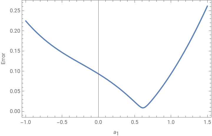
4.1 Manifold at q=2 cycles and order n=2
4.1 Manifold at cycles and order
q=2
n=2
In[]:=
ClearAll[alpha,beta];alpha[a1_]:=With[{a2=1-a1},1/12*a1^2-1/12*a1*a2-1/24*a2^2]beta[a1_]:=With[{a2=1-a1},-1/24*a1+1/12*a2]
In[]:=
ClearAll[Manifold]Manifold[a1val_]:=Sqrt[Abs[alpha[a1val]]^2+Abs[beta[a1val]]^2]
In[]:=
Plot[Manifold[a1],{a1,-1.0,1.5},PlotStyle->PointSize[0.015],Frame->True,FrameLabel->{"","Error"}]
a
1
Out[]=
Visualization
Visualization
Visualizations of the complete manifold and each contribution. The solver doesn’t know the difference between different points, which results in arbitrary indexing of the solutions. Due to this reason, the branch colors change at certain points.
Visualization
Visualization
Visualizations of the complete manifold and each contribution. The solver doesn’t know the difference between different points, which results in arbitrary indexing of the solutions. Due to this reason, the branch colors change at certain points. There are 2 free parameters at 5 cycles, which means we need to fix one of them for each plot in order to present how the manifold changes well.
5. Bibliography
5. Bibliography
[1] A. Arnal, F. Casas, and C. Chiralt, “A Note on the Baker–Campbell–Hausdorff Series in Terms of Right-Nested Commutators”, Mediterranean J. Math. 18, 53 (2021), arXiv:2006.15869 [math-ph].
[2] M. Suzuki, “Generalized Trotter’s Formula and Systematic Approximants of Exponential Operators and Inner Derivations with Applications to Many Body Problems”, Commun. Math. Phys. 51, 183–190 (1976).
[3] N. Hatano and M. Suzuki, “Finding Exponential Product Formulas of Higher Orders”, in Quantum annealing and other optimization methods (Springer Berlin Heidelberg, 2005), pp. 37–68.
[4] H. Yoshida, “Construction of higher order symplectic integrators”, Physics Letters A 150, 262–268, issn: 0375-9601 (1990).
[5] I. Omelyan, I. Mryglod, and R. Folk, “Optimized Forest–Ruth- and Suzuki-like algorithms for integration of motion in many-body systems”, Computer Physics Communications 146, 188–202 (2002).
[6] M. Maležič and J. Ostmeyer, Efficient Trotter-Suzuki schemes for Long-time Quantum Dynamics, 2601.18756.
[7] V. Shtabovenko, R. Mertig, and F. Orellana, “Feyncalc 10: do multiloop integrals dream of computer codes?”, Computer Physics Communications 306, 109357, issn: 0010-4655 (2025).
CITE THIS NOTEBOOK
CITE THIS NOTEBOOK
Efficient Trotter-Suzuki schemes for long-time quantum dynamics
by Marko Maležič, Johann Ostmeyer
Wolfram Community, STAFF PICKS, March 17, 2026
https://community.wolfram.com/groups/-/m/t/3665192
by Marko Maležič, Johann Ostmeyer
Wolfram Community, STAFF PICKS, March 17, 2026
https://community.wolfram.com/groups/-/m/t/3665192