CITE THIS NOTEBOOK: Modern Portfolio Theory by Jonathan Kinlay. Wolfram Community FEB 20 2023.
Extract from the upcoming book “Equity Analytics” by Jonathan Kinlay where complete materials will be available.
Extract from the upcoming book “Equity Analytics” by Jonathan Kinlay where complete materials will be available.
In 1952, Harry Markowitz introduced the concept of Modern Portfolio Theory through his doctoral thesis, commonly referred to as the Markowitz model. This theory is based on the idea that investors aim to maximize a portfolio' s expected return while considering a certain level of risk. Efficient portfolios, which meet this criterion, are those where achieving a higher expected return necessitates taking on more risk. As a result, investors must strike a balance between risk and expected return. The relationship between risk and expected return for efficient portfolios is illustrated by the efficient frontier, a graph that displays this trade - off. All efficient portfolios, represented as points on the efficient frontier, are diversified to minimize risk. In this chapter we review some of the core concepts of MTP and illustrate how to approach the portfolio optimization problem in the Wolfram Language.
Portfolio Construction
Portfolio Construction
We begin our exploration of the topic of modern portfolio theory by defining a universe of stocks comprising a random sample of 25 of the constituents of the S&P 500 index as a selected point in time:
In[]:=
startDate=DateObject[{2018,1,3}]
Out[]=
In[]:=
portfolioStocks=RandomSampleSelectEntity["Equities",#]&/@EntityMemberList,startDate,EntityQ,25//Sort;nstocks=Length@portfolioStocksportfolioStocks//Short
Out[]=
25
Out[]//Short=
,,,,,,,,,,,,,,,,,,,,,,,,
The RandomWeighting function is used to generate 10,000 different sets of weights that are applied to the stocks in the investment universe to create 10,000 different portfolios. All of the portfolio weights must lie in the range {0, 1}, i.e. we do not allow short sales and the sum of the weights must equal 1.0 (no leverage). We examine the annual return and volatility of these portfolios over the preceding 5 years.
In[]:=
wgts=RandomWeighting[10000,nstocks,1.0];
In[]:=
weights=Table[,{i,nstocks}];
ω
i
In[]:=
tsPortfolioReturns=PortfolioReturns[portfolioStocks,{2013,1,3},{2017,12,29}];
In[]:=
AbsoluteTiming[portfolioRiskReturn=ParallelTable[PortfolioRiskReturn[tsPortfolioReturns,weights/.weights->wgt],{wgt,wgts},Method->"CoarsestGrained"];]
Out[]=
{101.076,Null}
The result is an array of annual return and volatilities for each of the 10,000 portfolios:
In[]:=
portfolioRiskReturn[[1;;5,1;;2]]
Out[]=
{{0.127391,0.139031},{0.155703,0.138864},{0.130991,0.140689},{0.122654,0.133249},{0.121784,0.134468}}
Minimum Variance Portfolio
Minimum Variance Portfolio
We will shortly plot these results on a chart, but first we will use the FindMinimum function to identify the return and volatility of the portfolio having the minimum variance, amongst all the possible variations of allocation weightings.
In[]:=
{portfolioAverageReturns,portfolioVolatility}=Take[PortfolioRiskReturn[tsPortfolioReturns,weights],2];
In[]:=
portfolioConstraints=Total[weights]==1&&And@@(0<=#<=1&/@weights);(*Setconstraintsonweightstothattheumoftheweights=1andallweightslieintherange{0,1}*)
In[]:=
minVarPortfolio={portfolioVolatility,portfolioAverageReturns}/.FindMinimum[{portfolioVolatility,portfolioConstraints},weights][[2]]
Out[]=
{0.104783,0.0998676}
For completeness, we also find the volatility and return of the S&P 500 index over the same period
In[]:=
tsSP500Returns=EntityDailyReturns,{2013,1,3},{2017,12,29};
In[]:=
SP500RiskReturn=PortfolioRiskReturn[tsSP500Returns][[{2,1}]]
Out[]=
{0.118687,0.120999}
The Efficient Frontier
The Efficient Frontier
The efficient frontier comprises portfolios which, for a given level of risk, have the highest expected return and, conversely, for a given rate of return have the lowest volatility. We can identify portfolios lying on the frontier using the FindMinimum function to identify the allocation weights for portfolios that have the lowest volatility for a specified rate of return (in the range of 1% to 32%).
In[]:=
effFrontier=ParallelTable[{FindMinimum[{portfolioVolatility,portfolioConstraints&&portfolioAverageReturns==i},weights][[1]],i},{i,0.01,0.32,.02},Method->"CoarsestGrained"]//Quiet;
We will also compute the allocation weights for several portfolios on the frontier:
In[]:=
effFrontierWgts=ParallelTable[FindMinimum[{portfolioVolatility,Total[weights]==1&&portfolioAverageReturns==i&&And@@(0<=#<=1&/@weights)},weights][[2]],{i,0.15,0.30,.05},Method->"CoarsestGrained"]//Quiet;
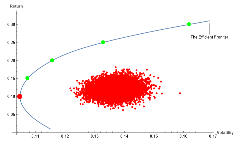
Finally, we are ready to combine all of the above information in a single plot that shows the efficient frontier, global minimum variance portfolio and other portfolios on the frontier and the collection of portfolios we created using random sets of allocation weights:
Composition of Portfolios on the Efficient Frontier
Composition of Portfolios on the Efficient Frontier
It is striking that none of the randomly generated portfolios lie close to the efficient frontier. That’s because the frontier portfolios typically have allocation weights that are “extreme”, with very large weights for some stocks and very small allocations to others. For example:
In[]:=
portfolio1=AssociationThread[portfolioStocks->Values@effFrontierWgts[[1]]]
Out[]=
0.00215412,0.0279105,0.0707088,0.0205041,0.0375922,0.175761,7.38827×,8.84198×,6.58751×,0.0102983,0.0000425169,0.0000209618,0.026013,0.0633854,0.0000269247,0.00567528,7.66668×,0.405446,0.0580264,3.98111×,7.00697×,0.00325516,0.0131276,0.00288251,0.077128
-6
10
-6
10
-6
10
-6
10
-6
10
-6
10
In[]:=
PieChart3D[portfolio1,ChartLegends->Placed[Automatic,Right],SectorOrigin->{Automatic,1}]
Out[]=


Performance of Portfolios on the Efficient Frontier
Performance of Portfolios on the Efficient Frontier
Because the allocation weights have been optimized so that efficient portfolios provide the maximum expected returns for a given level of risk, the equity curve of compounded returns is relatively smooth and monotonic and the portfolios easily outperform the S&P500 index over the formation period from 2013-2017:
In[]:=
tsPortReturns=PortfolioReturns[tsPortfolioReturns,Values@effFrontierWgts]
Out[]=
TimeSeries


In[]:=
DateListPlot[{CompoundReturn[tsPortReturns],CompoundReturn[tsSP500Returns]},Filling->Axis,PlotLabels->Join[Table[StringJoin["Portfolio ",ToString[i]],{i,4}],{" SP500"}],ImageSize->Large,PlotRange->All]
Out[]=
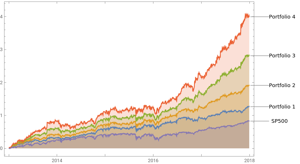
When we evaluate portfolio performance after the formation period, however, the story is very different. Although efficient portfolios outperform the S&P500 over the period from 2018-2022, there are times when they under-perform the index and the equity curve suffers from several large periodic declines lasting for several days, or weeks. This is the result of the extreme allocation profile of the portfolios, which entails making several large bets on stocks such as PEP and CME, which performed well during the formation period, but did much less well in the subsequent period from 2018. This variability in performance is a typical characteristic of portfolios constructed by mean-variance optimization.
For this reason equity portfolio managers will typically impose additional constraints on the allocation weights, to avoid over- or under-weighting specific stocks or industry sectors, with the aim of constructing portfolios that perform more robustly out of sample.
For this reason equity portfolio managers will typically impose additional constraints on the allocation weights, to avoid over- or under-weighting specific stocks or industry sectors, with the aim of constructing portfolios that perform more robustly out of sample.
In[]:=
tsSP500Returns=EntityDailyReturns,{2018,1,3},{2022,12,30}
Out[]=
TimeSeries

In[]:=
tsPortfolioReturns=PortfolioReturns[portfolioStocks,{2018,1,3},{2022,12,30}];
In[]:=
tsPortReturns=PortfolioReturns[tsPortfolioReturns,Values@effFrontierWgts]
Out[]=
TimeSeries
Dynamics of the Efficient Frontier
Dynamics of the Efficient Frontier
One of the major challenges in portfolio construction is that the temporal variability in asset returns and covariances induces substantial change in the shape of the efficient frontier. This means that the composition of a portfolio with a specific risk-return profile is liable to alter significantly over time. Furthermore, the volatility of an optimal portfolio with a specific rate of expected returns will likewise be subject to substantial variation. To illustrate this effect, we estimate the efficient frontier for our universe of 25 stocks for six years, using daily returns data for the prior five years in each case.
Depending on the year in question, we observe that an optimal portfolio with an expected return of, say, 12% per year, might have an estimated annual volatility of as low as 7% (in 2015) to as high as 12% (in 2019).
Depending on the year in question, we observe that an optimal portfolio with an expected return of, say, 12% per year, might have an estimated annual volatility of as low as 7% (in 2015) to as high as 12% (in 2019).
Notes
Notes