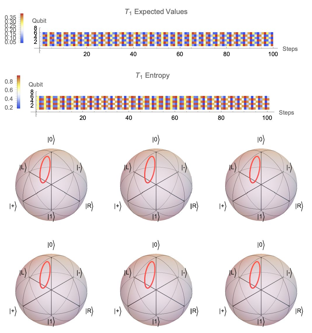
Quantum information systems are challenging to visualise since the dimension of the space grows exponentially with the number of qubits. However, by extracting information about a quantum state, we can more easily visualise meaningful qualities of the system. This project focuses on the iterative flow of information through cellular-automata-like quantum circuits.
Packages
Packages
Initialisation
Initialisation
Introduction
Introduction
Approach and Implementation
Approach and Implementation
This project is inspired by the paper “Entangled quantum cellular automata, physical complexity, and Goldilocks ”. In the paper, the authors examine quantum circuits composed of gates controlled by the adjacent qubits; the quantum analogue to cellular automata rules.
For example, we can consider a Hadamard gate that is activated by the condition that the two adjacent qubits are in. The quantum circuit would look like:
[1]
rules
For example, we can consider a Hadamard gate that is activated by the condition that the two adjacent qubits are in
state
|0〉
Out[]=
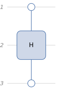
where an empty circle denotes that the qubit should be in state for the gate to be activated and, equivalently, a filled circle denotes a .
|0〉
|1〉
This circuit would transform
Out[]=

and leave all other possible states unchanged.
In general, a gate that acts on qubit will be of the form
In general, a gate that acts on qubit
j
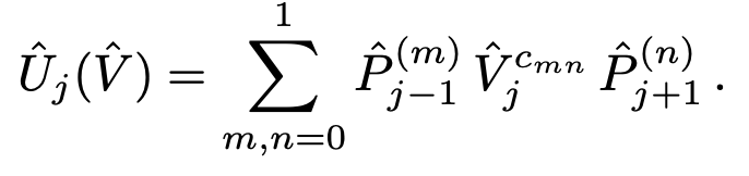
where is the unitary to be applied, ∈{0,1} denotes whether should be applied when qubit matches and qubit matches , and the s are the control operators. In Mathematica, we can implement this as
V
c
mn
V
j+1
|n〉
j-1
|m〉
P
UjCircuit[{RR_,v_},{site_,graph_}, label_String]:=Module[{adj,cmn},adj=AdjacencyList[graph,site];cmn=Reverse@IntegerDigits[RR,2,4];QuantumCircuitOperator[MapIndexed[If[#1==1,{"C",v->site,#2[[1]]-1,adj},Nothing]&,cmn], "Label"->label]]
The parameters are:
◼
RR: a number corresponding to a classical cellular automata rule (based on the paper, we will take its base-2 form)
◼
v: operator to be applied if activated.
◼
site: qubit site where v is applied.
◼
graph: graph yielding required relation between the sites.
In the paper, the authors mainly focus on two cellular automata rules which they label and . The rule is characterised by activating the effect of an operator at a qubit site if both of the adjacent qubits are in . This rule is implemented above with the operator v being a Hadamard gate. The rule has the effect that an operator is applied at a qubit site only if the adjacent qubits are different. This is illustrated bellow with a Hadamard gate.
T
1
T
6
T
1
k
|0〉
T
6
Out[]=
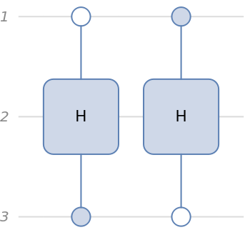
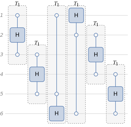
To form the circuits, we must decide in what order to apply the gates. In this project, we choose to first apply the gates to the even qubits and then the odd qubits, adding cyclic boundary conditions. For instance, the circuit would look like, for and respectively,
T
1
n6
n7
◼
n6
◼
n6
Out[]=
◼
n7
◼
n7
Out[]=
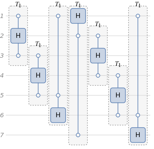
We concentrate on these two rules and how we can visualise the iterative evolution,of an initial state through these kinds of circuits. That is, we keep feeding through the resulting state to the circuit and examine certain properties that describe how the state evolves.
Theoretical Background
Theoretical Background
This projet focuses on specific properties of the quantum states as opposed to descriptions in the complete Hilbert space. In particular, we will explore the expected value, the Von Neumannm entropy with respect to the rest of the qubits, and the reduced state associated with each qubit. By the reduced state, we mean the state left after tracing out all but one of the qubits. That is, we think of each qubit belonging to a local observer whom can only measure that one qubit and so cannot see correlations, thus only being able to see the reduced state of the qubit. From these reduced states we would be able to recover the expected value and entropy associated with the respective qubit.
Now, the notion of expected value is usually clear and unambiguous. However, this is often not the case for entropy. This term is famously ambiguous and was popularised in information theory by Claude Shannon, he explains in (McIrvine and Tribus 1971):
My greatest concern was what to call it. I thought of calling it ‘information,’ but the word was overly used, so I decided to call it ‘uncertainty.’ When I discussed it with John von Neumann, he had a better idea. Von Neumann told me, ‘You should call it entropy, for two reasons. In the first place your uncertainty function has been used in statistical mechanics under that name, so it already has a name. In the second place, and more important, no one really knows what entropy really is, so in a debate you will always have the advantage.’
For our purposes, we interpret the Von Neumann entropy to quantify the entanglement of pure and mixed bipartite quantum. More concretely, if one of the qubits has entropy 0, measuring it tells us no information about the rest of the system as it is separable from it and we say the system is in a pure state with respect to that qubit. The higher the entropy of a qubit is the more entangled the qubit is with that system and the more information we would find out.
Take for example the Bell State,
Now, the notion of expected value is usually clear and unambiguous. However, this is often not the case for entropy. This term is famously ambiguous and was popularised in information theory by Claude Shannon, he explains in (McIrvine and Tribus 1971):
My greatest concern was what to call it. I thought of calling it ‘information,’ but the word was overly used, so I decided to call it ‘uncertainty.’ When I discussed it with John von Neumann, he had a better idea. Von Neumann told me, ‘You should call it entropy, for two reasons. In the first place your uncertainty function has been used in statistical mechanics under that name, so it already has a name. In the second place, and more important, no one really knows what entropy really is, so in a debate you will always have the advantage.’
For our purposes, we interpret the Von Neumann entropy to quantify the entanglement of pure and mixed bipartite quantum
[2]
states
Take for example the Bell State,
Out[]=
1
2
1
2
when you measure one of the qubits, you are guaranteed to obtain the same result when you measure the other qubit.
Visualisations
Visualisations
We can either think of the initial state evolving discretely or continuously.
We call discrete evolution of the state the successive application of a quantum circuit to an initial state. We visualise this by calculating a property of each qubit at each iteration, assigning a colour to the result and plot them in columns one after the other. The two properties explored in this project are the expected value of a measurement performed on each qubit and the entropy of each qubit with respect to the rest as a measure of how entangled it is. What interesting patterns should we expect to arise in this evolution? Should we expect something periodic? Should we expect the system to thermalise, that is, that it is equally likely for each qubit to be in either state? These are the questions we will explore with the visualisations.
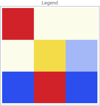
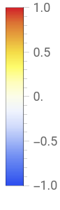
In this project, we associate qubit with a measurement of -1 and qubit with a measurement of 1. When plotting the expected values of the qubits, we use the following colour palette:
In this project, we associate qubit
|0〉
|1〉
Out[]=
We shall also consider a smoothed out evolution of the initial state. We can smooth out this evolution by considering “fractional” applications of the quantum circuit. This allows us to consider the position of each qubit in the Bloch sphere over time as we have a smooth transition between each complete application of the circuit.
An Illustrative Example
An Illustrative Example
Before diving into many-qubits systems, let us first illustrate the process with a small number of them.
Setup
Setup
First, we build the circuit.
Generate the operators for the circuit
To speed things up we transform the circuit into a single unitary matrix that we can apply to the initial state.
Evolution
Evolution
◼
Results
We present the evolution of the initial state up to the 150th application of the circuit split into three rows.
We observe two main qualities. We see that the middle four qubits do not change, the middle two always yielding a measurement of 1 and qubits 3 and 5 always yielding a measurement of -1. The other quality is that the pattern seems to repeat, albeit up to some precision. Indeed, using FindTransientRepeat with a tolerance of up to 0.1, the function finds that the first 203 columns form the repeating pattern.
We also plot the entropy of the qubits and similarly find that there seems to be a repeating pattern, split into three rows again.
We also notice how the middle four qubits are redundant information in the system since they have zero entropy.
◼
Results
The fact that we see a closed orbit, and keep seeing it for higher number of iterations, implies that the evolution of this initial state is periodic. However, one must be mindful that this is a visual explanation and so is prone to error, it could be the case that the orbit simply deviates ever so slightly from the trajectory we see, and so the orbit is not perfectly periodic after all.
The Mathematical Explanation
The Mathematical Explanation
The only way we can be sure whether the behaviour shown previously is periodic is by diving into the mathematical properties of the unitary matrix representing the quantum circuit. It is also worth wondering, should we expect periodic behaviour or is this surprising?
Suppose we have (not normalised),
where
This happens if and only if
Let us see an example. First, let us look at the list of eigenvalues, in complex polar coordinates, of the circuit.
This doesn’t look promising as most of the eigenvectors have a nonzero coefficient and so would yield a really high period. For the sake of simplicity, let’s chop the values that are too small.
This is looking better. What eigenvalues do these eigenvectors have?
Surprisingly, or perhaps unsurprisingly, the eigenvectors with higher weights either have eigenvalue 1 or an eigenvalue where the denominator of the phase is the same, 171. Thus, we should expect this state to have a relatively small period.
How accurate is this? Well, if we compute the resulting vector after chopping off the small coefficients, we get
which is very accurate, specially as the expected value involves the amplitudes squared.
As a last point, we note the enormity of the number of applications of the circuit if we wanted to get periodic evolution for any initial state.
This is in the order of billions of times even for the low precision eigenvalues. So, we can conclude that not all initial conditions have periodic evolution.
Why Mathematics is Cool
Why Mathematics is Cool
Maths’ only benefit is not just providing rigour to our explanations. Maths sets out the foundations to carve out interesting patterns from seemingly bland phenomena. For instance, as is often the case with problems involving matrices, in the previous section we realised we were looking at the problem with the wrong basis - from the wrong perspective. Now that we know what the natural basis of the problem is, here is what we can do:
◼
Results
◼
State
◼
State
Compilation of Results
Compilation of Results
Whilst it would have been insightful to carry out a similar mathematical analysis as above for bigger spaces, the fact that the computational complexity of quantum systems grows exponentially makes this extremely difficult. Instead, we provide a compilation of interesting results and patterns that emerge from the experiments.
◼
Evolution
◼
Evolution
◼
Evolution
◼
Evolution
◼
Evolution
◼
Evolution
◼
Evolution
◼
Evolution
Concluding Remarks
Concluding Remarks
We can conclude that cellular-automata like circuits do not necessarily produce periodic evolution and that the natural way to approach this phenomenon is by using the orthonormal basis induced by the unitary matrix associated with the quantum operator. Nonetheless, the emergent patterns are interesting and worth of study, with potential relation to number theory and almost-rational numbers.
Acknowledgments
Acknowledgments
I would like to thank my mentors Gianmarco Morbelli and Nikolay Murzin for their support and guidance during the development of this project, as well as Sebastian Rodriguez and Daniel Sanchez for their expertise in the Wolfram Language, and Mads Bahrami for his help on the theoretical background of quantum mechanics. I would also like to thank Stephen Wolfram for suggesting this project. I also extend my gratitude to Dr. Roy Moulik for instilling in me a passion for Quantum Information Theory.
I would like to thank my mentors Gianmarco Morbelli and Nikolay Murzin for their support and guidance during the development of this project, as well as Sebastian Rodriguez and Daniel Sanchez for their expertise in the Wolfram Language, and Mads Bahrami for his help on the theoretical background of quantum mechanics. I would also like to thank Stephen Wolfram for suggesting this project. I also extend my gratitude to Dr. Roy Moulik for instilling in me a passion for Quantum Information Theory.
References
References
1
.S. Chehade and A. Vershinina, (2019), “Quantum entropies”, Scholarpedia. http://www.scholarpedia.org/article/Quantum_entropies#von_Neumann_entropy
2
.W. Fedus, (2017),”Entropy in Classical and Quantum Information Theory”, https://acsweb.ucsd.edu/~wfedus/pdf/courses/210a_assignment.pdf
Cite This Notebook
Cite This Notebook