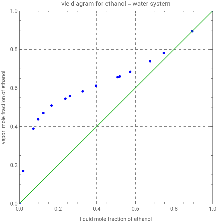
The code fits a thermodynamic model to experimental vapor-liquid equilibrium (VLE) data for the ethanol-water system at atmospheric pressure. The script begins by loading a dataset of 17 experimental points containing liquid mole fraction (x), vapor mole fraction (y), and boiling temperature (T in °C) for ethanol, then extracts these into separate vectors and plots the raw experimental x-y data against the y=x diagonal (which represents the no-separation reference line for distillation). Two correlations are then defined: the Antoine equation, which predicts the pure-component vapor pressure of ethanol and water as a function of temperature, and the Van Laar activity coefficient model, which uses two binary interaction parameters (A12 and A21) to capture the non-ideal mixing behavior between the two components.
The core of the program is the myvle function, which solves the modified Raoult’s law equilibrium equations simultaneously for vapor composition (y) and temperature (T) at each given liquid composition (x), using FindRoot. A Fitness function is then defined as the sum of squared errors between the model’s predicted (y, T) values and the experimental (y, T) values — this is the objective function that needs to be minimized by adjusting A12 and A21.
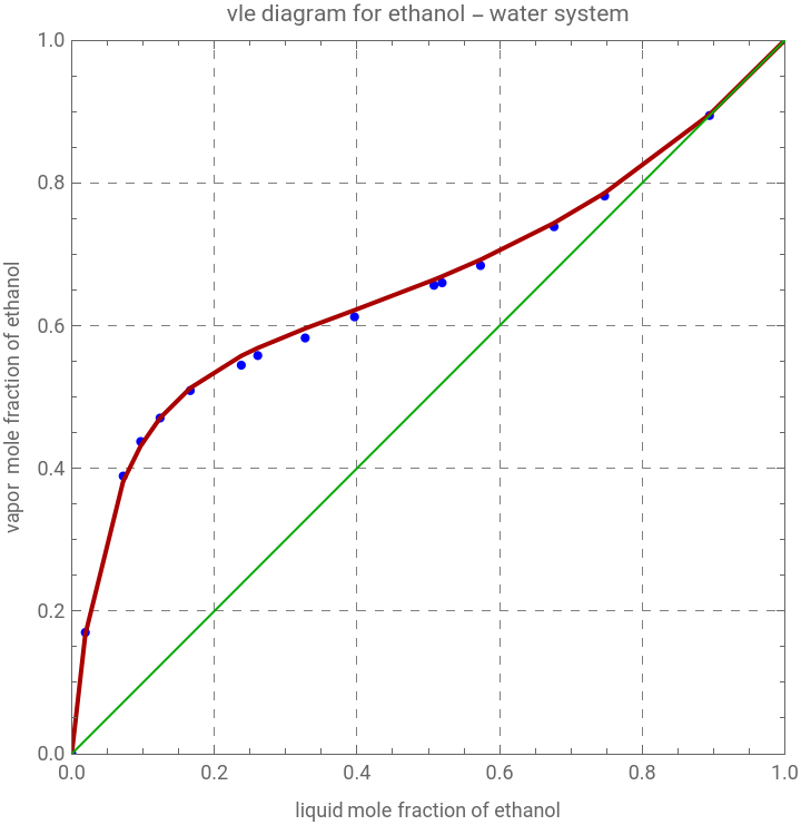
To find the optimal Van Laar parameters, the code implements a custom Particle Swarm Optimization (PSO) algorithm from scratch rather than using a built-in solver like NMinimize. The psoOptimize function initializes a swarm of 500 candidate solutions (particles) randomly within bounds [0.1, 2] for the two parameters, then iteratively updates each particle’s velocity and position based on its own best-known position (pbest) and the swarm’s global best position (gbest), using standard PSO inertia/cognitive/social coefficients (w, c1, c2). After running 100 iterations, the algorithm converges to A12 ≈ 1.63575 and A21 ≈ 0.939407 with a final loss of ~0.324831, and the resulting fitted curve is overlaid in red on the original experimental plot, showing a close match to the measured VLE behavior, including the characteristic curvature near the azeotropic region around x ≈ 0.89.
Ethanol-Water VLE Data at 1 atm
Columns:X_EtOH (liquid),Y_EtOH (vapor),T (°C)
Columns:X_EtOH (liquid),Y_EtOH (vapor),T (°C)
vleData={{0.0,0.0,100.0},{0.019,0.17,95.5},{0.0721,0.3891,89.0},{0.0966,0.4375,86.7},{0.1238,0.4704,85.3},{0.1661,0.5089,84.1},{0.2377,0.5445,82.7},{0.2608,0.558,82.3},{0.3273,0.5826,81.5},{0.3965,0.6122,80.7},{0.5079,0.6564,79.8},{0.5193,0.6599,79.7},{0.5732,0.6841,79.3},{0.6763,0.7385,78.74},{0.7472,0.7815,78.41},{0.8943,0.8943,78.15},{1.0,1.0,78.3}};
Extract columns
xEtOH=vleData[[All,1]];yEtOH=vleData[[All,2]];tempC=vleData[[All,3]];
Plot Psat vs T
plt1=ListPlot[Transpose@{xEtOH,yEtOH},PlotStyle->{Blue,Thick},Frame->True,FrameLabel->{"liquid mole fraction of ethanol","vapor mole fraction of ethanol"},PlotLabel->"vle diagram for ethanol - water system",GridLines->Automatic,GridLinesStyle->Directive[Gray,Dashed],AspectRatio->1,PlotRange->{{0,1},{0,1}},Epilog->{Darker@Green,Line[{{0,0},{1,1}}]}]
Out[]=
Antoine Equation where Temperature in °C and Pressure in mmHg
Psat1[t_]:=10^(8.20417-1642.89/(230.3+t));(*Ethanol*)Psat2[t_]:=10^(8.07131-1730.63/(233.426+t));(*Water*)
van Laar Model
gamma1[A12_,A21_,x_]:=Exp[A12(A21(1-x)/(A12x+A21(1-x)))^2];gamma2[A12_,A21_,x_]:=Exp[A21(A12x/(A12x+A21(1-x)))^2];
In[]:=
P=760;
In[]:=
myvle[A12_,A21_]:=Module[{i,system,sol,x,t,y},(*Systemofequationsforxandydetermination*)system[x_]:={Py==gamma1[A12,A21,x]*Psat1[t]x,gamma1[A12,A21,x]*Psat1[t]x+gamma2[A12,A21,x]*Psat2[t](1-x)==P};i=1;While[i<=17,{x=xEtOH[[i]];sol[i]=Quiet@FindRoot[system[x],{t,95},{y,0.5},MaxIterations->1000];i++}];Table[{y,t}/.sol[i],{i,1,17}]]
SwarmDim=2;(*3Dproblem*)(*upperandlowerboundsfothesearchdomain*)FitnessLB=0.1;FitnessUB=2;c1=1.42;c2=1.42;w=0.72984;(*psoparameters*)T=tempC;Fitness[{A12_,A21_}]:=Module[{tbl},tbl=myvle[A12,A21];Sum[(tbl[[i]][[1]]-yEtOH[[i]])^2+(tbl[[i]][[2]]-tempC[[i]])^2,{i,1,Length@tempC}]]
In[]:=
Clear[A12,A21]
PSO Optimizer
psoOptimize[lossFunc_,dim_,lb_,ub_,nParticles_:500,nIter_:50,w_:0.72984,c1_:2,c2_:2]:=Module[{particles,velocities,pbest,pbestScore,gbest,gbestScore,convergence={},r1,r2,score,gbestIdx},(*Initializeparticlesuniformlywithin[lb,ub]ineachdimension*)particles=RandomReal[{lb,ub},{nParticles,dim}];velocities=ConstantArray[0.,{nParticles,dim}];pbest=particles;pbestScore=Table[lossFunc[particles[[i]]],{i,nParticles}];gbestIdx=First@Ordering[pbestScore,1];gbestScore=pbestScore[[gbestIdx]];gbest=pbest[[gbestIdx]];Do[Do[r1=RandomReal[1,dim];r2=RandomReal[1,dim];velocities[[i]]=w*velocities[[i]]+c1*r1*(pbest[[i]]-particles[[i]])+c2*r2*(gbest-particles[[i]]);particles[[i]]+=velocities[[i]];(*keepparticleswithinbounds*)particles[[i]]=Clip[particles[[i]],{lb,ub}];score=lossFunc[particles[[i]]];If[score<pbestScore[[i]],pbest[[i]]=particles[[i]];pbestScore[[i]]=score;];,{i,nParticles}];gbestIdx=First@Ordering[pbestScore,1];gbestScore=pbestScore[[gbestIdx]];gbest=pbest[[gbestIdx]];AppendTo[convergence,gbestScore];If[Mod[t,10]==0,Print["PSO Iter ",t," Loss = ",gbestScore]];,{t,nIter}];{gbest,gbestScore,convergence}];
Run PSO
{bestPos,bestScore,convergence}=psoOptimize[Fitness,SwarmDim,FitnessLB,FitnessUB,50,100,w,c1,c2];Print["Best position: ",bestPos];Print["Best fitness: ",bestScore];
PSO Iter 10 Loss = 0.341344
PSO Iter 20 Loss = 0.324998
PSO Iter 30 Loss = 0.324927
PSO Iter 40 Loss = 0.324832
PSO Iter 50 Loss = 0.324831
PSO Iter 60 Loss = 0.324831
PSO Iter 70 Loss = 0.324831
PSO Iter 80 Loss = 0.324831
PSO Iter 90 Loss = 0.324831
PSO Iter 100 Loss = 0.324831
Best position: {1.63575,0.939407}
Best fitness: 0.324831
Best position = {1.63575,0.939407}
A12=1.6798;A21=0.9227;(*binaryinteractionparametersfromlitterature*)Fitness[{A12,A21}]
Out[]=
0.485212
In[]:=
myvle[bestPos[[1]],bestPos[[2]]]
Out[]=
{{0.,99.9968},{0.167347,95.4576},{0.381997,88.6834},{0.431425,86.9637},{0.470509,85.5755},{0.512418,84.0848},{0.557522,82.5409},{0.568551,82.1859},{0.59593,81.3668},{0.621599,80.6984},{0.664191,79.8175},{0.668873,79.7369},{0.692208,79.3776},{0.743708,78.7975},{0.785712,78.4946},{0.895622,78.1901},{1.,78.3192}}
In[]:=
yfit=Transpose[myvle[bestPos[[1]],bestPos[[2]]]][[1]]
Out[]=
{0.,0.167347,0.381997,0.431425,0.470509,0.512418,0.557522,0.568551,0.59593,0.621599,0.664191,0.668873,0.692208,0.743708,0.785712,0.895622,1.}
In[]:=
mydata=Transpose[Join[{xEtOH},{yfit}]]
Out[]=
{{0.,0.},{0.019,0.167347},{0.0721,0.381997},{0.0966,0.431425},{0.1238,0.470509},{0.1661,0.512418},{0.2377,0.557522},{0.2608,0.568551},{0.3273,0.59593},{0.3965,0.621599},{0.5079,0.664191},{0.5193,0.668873},{0.5732,0.692208},{0.6763,0.743708},{0.7472,0.785712},{0.8943,0.895622},{1.,1.}}
In[]:=
Show[plt1,ListPlot[mydata,PlotStyle->Darker@Red,Joined->True]]
Out[]=
CITE THIS NOTEBOOK
CITE THIS NOTEBOOK
van Laar equation parameters for ethanol-water system via particle swarm optimization
by Housam Binous
Wolfram Community, STAFF PICKS, June 29, 2026
https://community.wolfram.com/groups/-/m/t/3740710
by Housam Binous
Wolfram Community, STAFF PICKS, June 29, 2026
https://community.wolfram.com/groups/-/m/t/3740710