Quantum Cellular Automata (QCA) are promising examples of universal quantum systems [1][2][3]. If QCA could be created as physical systems, they could offer solutions to the problem of scaling up quantum computation to larger numbers of qubits. Here we explore QCA architectures in the Wolfram Language using the Quantum Framework paclet, develop a visualization technique for qubit arrays in QCA, and evaluate various interesting QCA models.
Working with Quantum Circuits and the Quantum Paclet
Working with Quantum Circuits and the Quantum Paclet
Clear and install the Quantum Framework Paclet:
In[]:=
PacletUninstall/@PacletFind["Quantum*"];
In[]:=
ClearAll["*QuantumFramework*","Wolfram`QuantumFramework`*","Wolfram`QuantumFramework`**`*"];
In[]:=
PacletInstall[ResourceObject["Wolfram/QuantumFramework"],ForceVersionInstall->True]
Out[]=
PacletObject

In[]:=
<<Wolfram`QuantumFramework`
Quantum computing offers a unique generalization of classical computing. Built off of a similar gate architecture to classical computing, quantum computing relies on the quantum behavior of particles to perform computation. Because quantum computation is built off of reversible, physical interactions between particles rather than interactions between clone-able classical signals, there are substantial differences between the gates used in quantum computation with those used in classical computation. Most notably, since all quantum gates are unitary and therefore must have the same number of input qubits as output qubits, quantum computation uses a different set of fundamental gates to classical logic. Classical AND and OR logic can be constructed in a quantum framework, and in fact can be constructed from the Fredkin (controlled swap) gate. However, because the Fredkin gate doesn't strictly have an "AND" output, instead having 3 output channels, and since the Fredkin gate only performs the AND operation when a particular input is set to , the Fredkin gate is not considered to be an AND gate. As far as 2 qubit logic goes, other gates such as RootSWAP, CX (aka CNOT), CY and CZ are the primary gates in the quantum framework.
|0〉
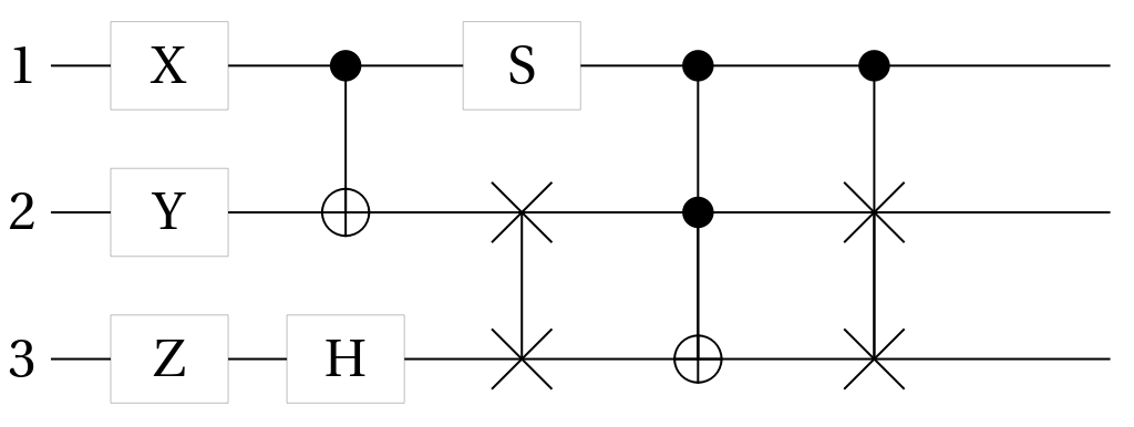
Some examples of Quantum Gates:
In[]:=
QuantumCircuitOperator[{QuantumOperator["X"],QuantumOperator["Y",{2}],QuantumOperator["Z",{3}],QuantumOperator["H",{3}],QuantumOperator["CNOT"],QuantumOperator["SWAP",{2,3}],QuantumOperator["S"],QuantumOperator["Toffoli"],QuantumOperator["Fredkin"]}]["Diagram"]
Out[]=
What is a Quantum Cellular Automaton?
What is a Quantum Cellular Automaton?
Quantum cellular automata can be understood as quantum analogues of classical cellular automata. In a classical cellular automaton, a regular arrangement of cells is populated with state information, and repeatedly updated with a given rule. While this relies on a large space of cells and many update rules, it remains a simple system because of space and time invariances. The system can be decomposed into micro-scale behavior. Quantum cellular automata operate under similar principals, with a simple update rule repeated spatially and temporally across the automaton.
Exploring QCA Structures: Classical Analogues
Exploring QCA Structures: Classical Analogues
Because QCA are necessarily reversible, irreversible classical CA rules cannot be implemented in QCA. This also means that there is no direct equivalence between Wolfram ECA and QCA. As such, other classical models must be explored as a framework for QCA. I'm particularly interested in classical frameworks for QCA which express complex (Class 4) behavior, in hopes that the classical structure would carry over to useful quantum computation.
As a result of the no-cloning theorem, unlike classical computation, QCA rules cannot be performed in parallel since non-trivial rules do not commute. Instead, one scheme to avoid this is by staggering overlapping operations on different clock cycles, like a Margolus automaton. https://arxiv.org/pdf/quant-ph/0405174.pdf
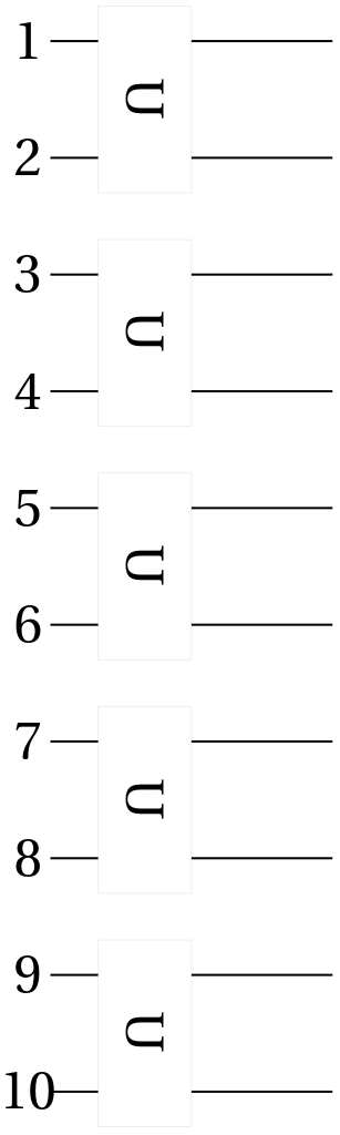
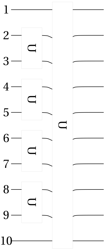
Note that the operator stretched across all of the channels only interacts with the first and last qubits.
To implement a classical Margolus automaton in the Wolfram Language, we define our steps where we partition the row into pairs and apply a rule on each pair of cells, and iterate over these steps with NestList.
For each input pair of elements, look up a unique output pair:
In[]:=
evenElementsMargolus[list_List,rule_List]/;Length[rule]==4:=Flatten[Map[rule[[FromDigits[#,2]+1]]&,Partition[list,2]]]
Alternate pairings:
In[]:=
oddElementsMargolus[list_List,rule_List]/;Length[rule]==4:=Flatten[Map[rule[[FromDigits[#,2]+1]]&,Partition[list,2,2,{2,2}]]]//RotateLeft
To make it easier to iterate over these automata for visualization, the rules are canonicalized and assigned indices:
In[]:=
evenElementsMargolus[list_List,rule_Integer:0]:=evenElementsMargolus[list,Map[IntegerDigits[#,2,2]&,Permutations[{0,1,2,3},{4}][[rule]]]]
In[]:=
oddElementsMargolus[list_List,rule_Integer:0]:=oddElementsMargolus[list,Map[IntegerDigits[#,2,2]&,Permutations[{0,1,2,3},{4}][[rule]]]]
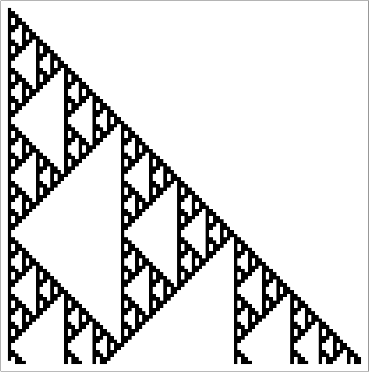
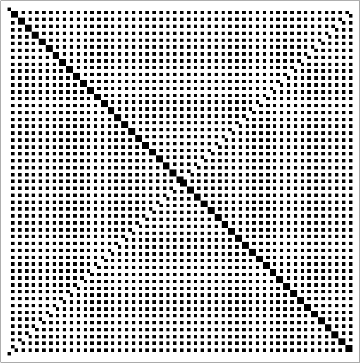
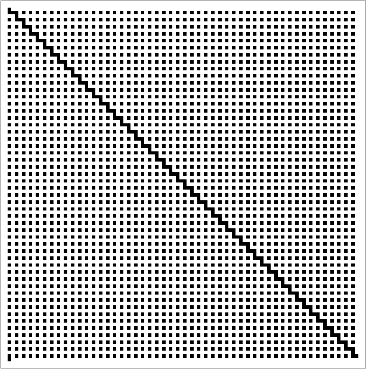
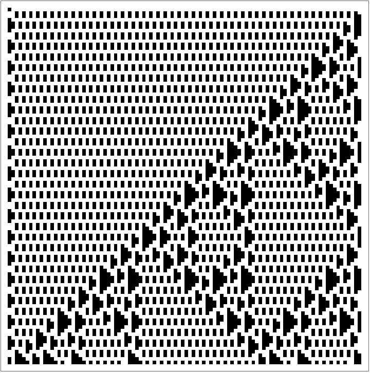
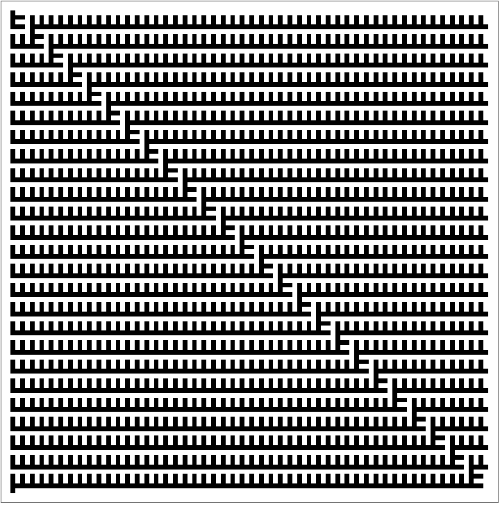
Draw all of the patterns generated by symmetric rules (same operation on even and odd steps):
In[]:=
Partition[Array[Function[{index},ArrayPlot[First/@NestList[{If[Divisible[i,2],evenElementsMargolus[#[[1]],index],oddElementsMargolus[#[[1]],index]],i++}&,{PadRight[{1},100],i=0},100]]],24],4]//Grid
Out[]=

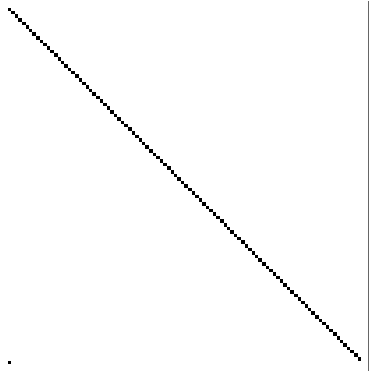
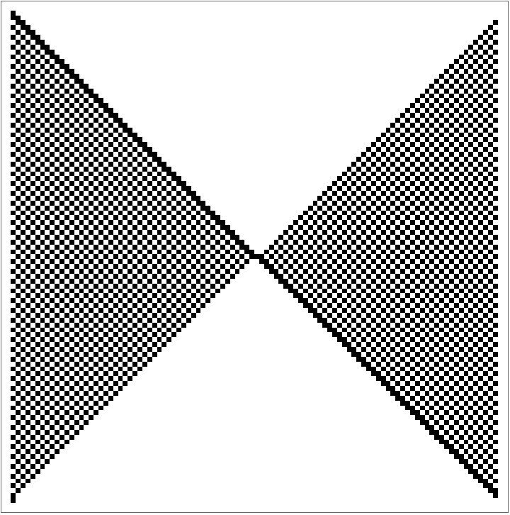
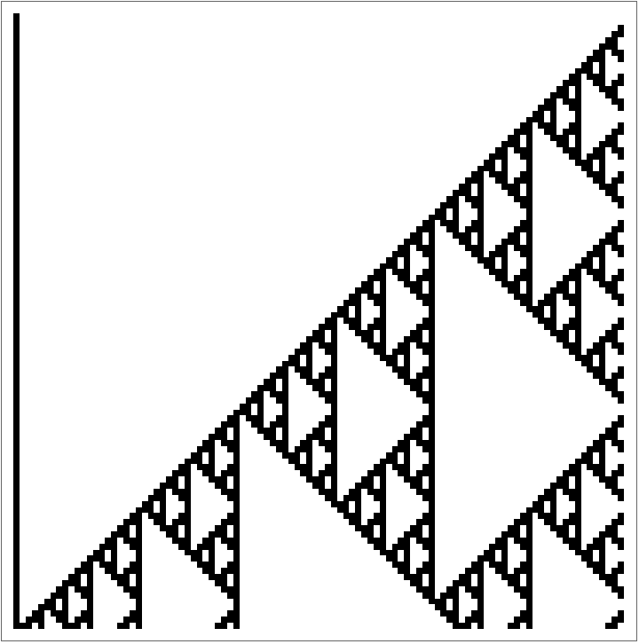
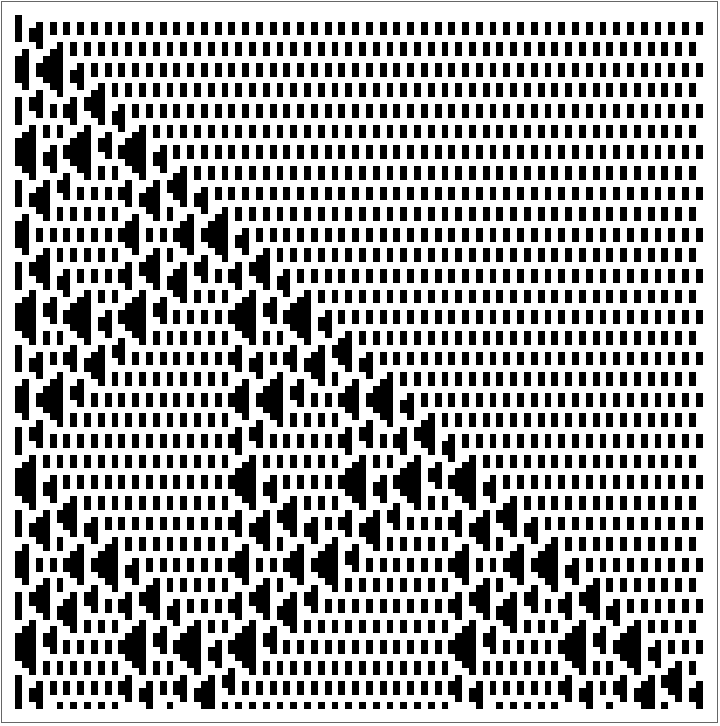
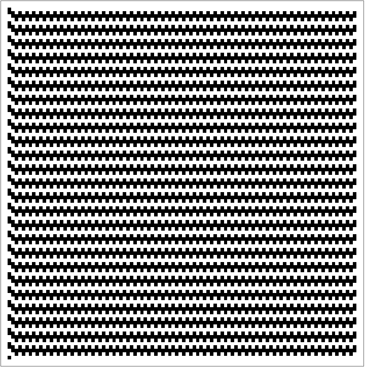
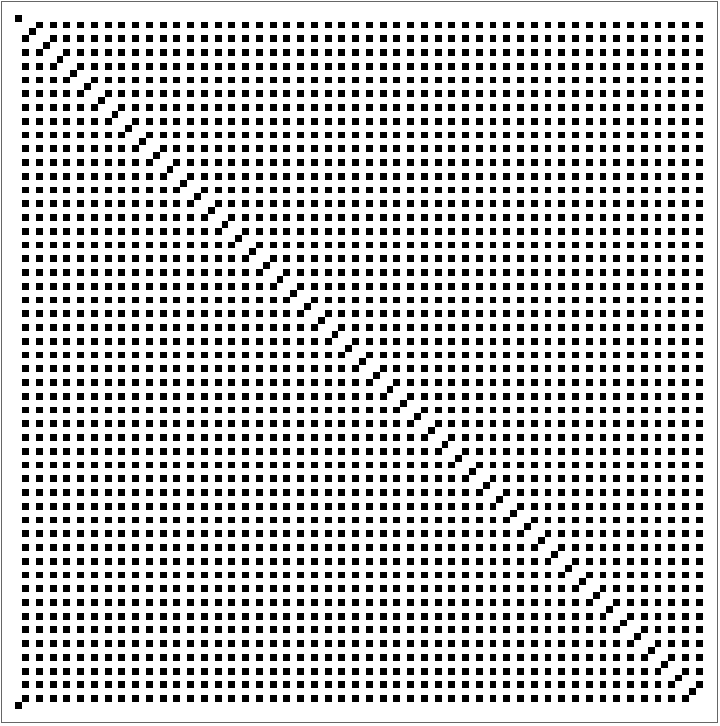
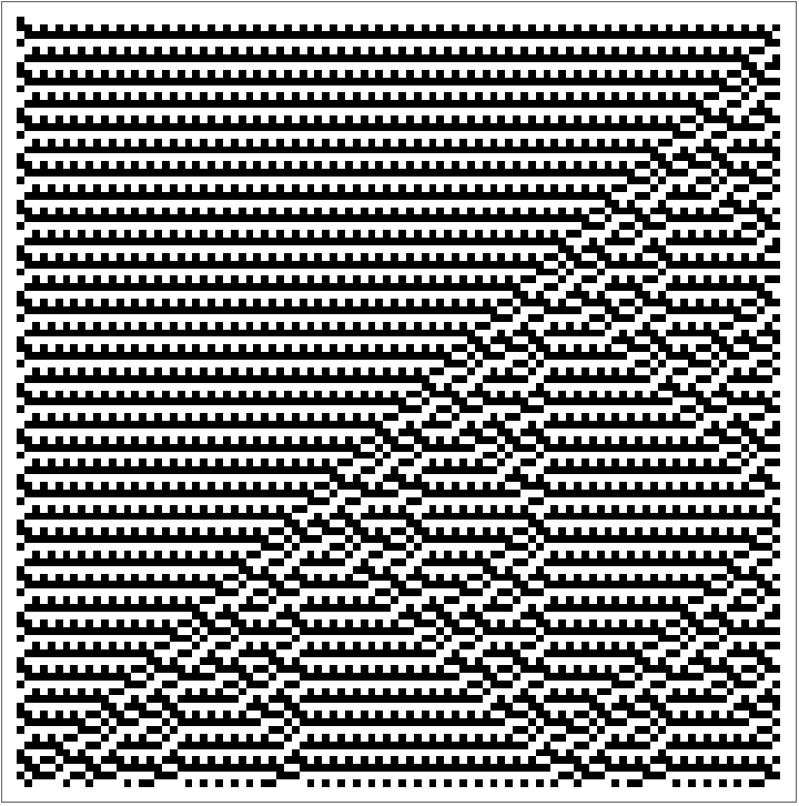
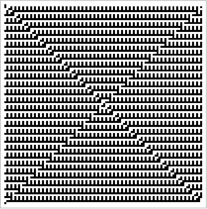
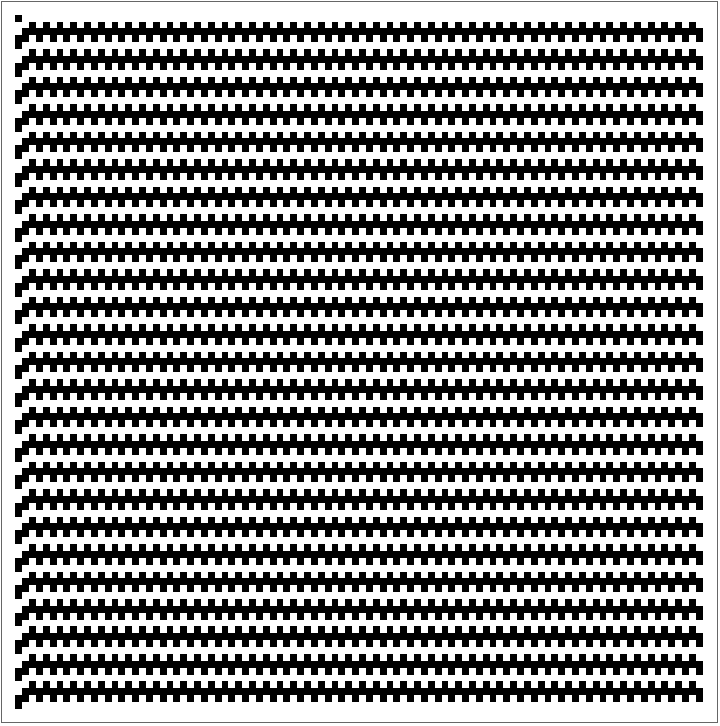
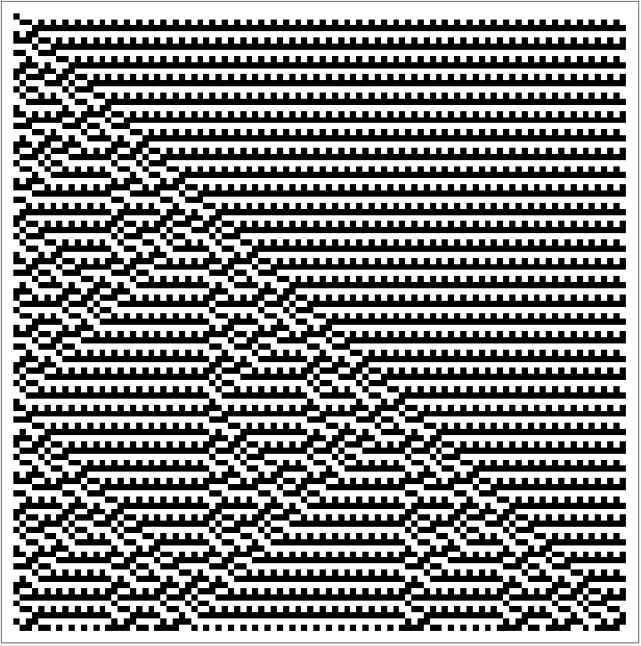
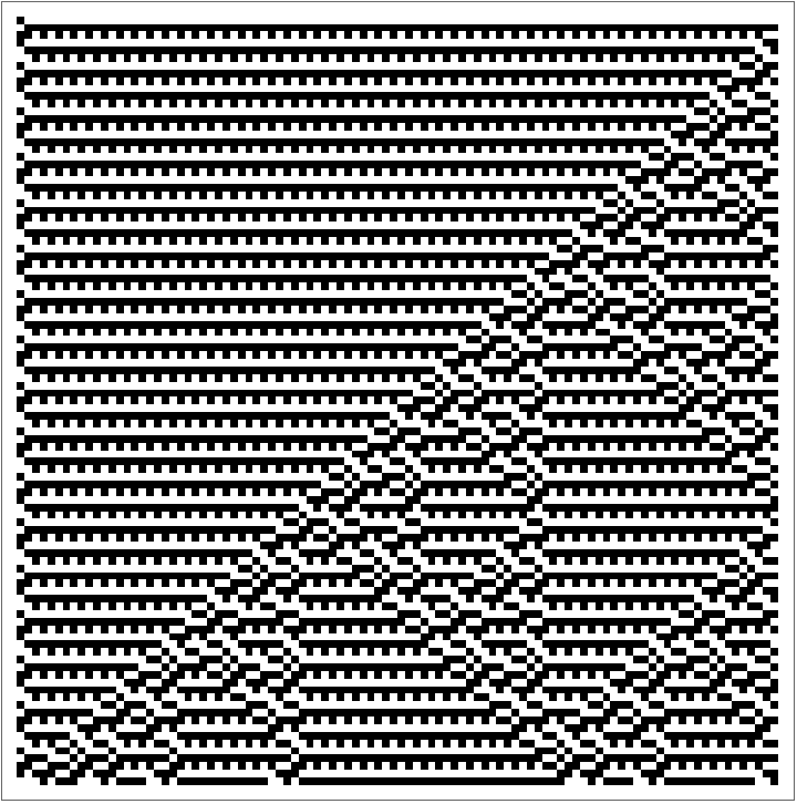
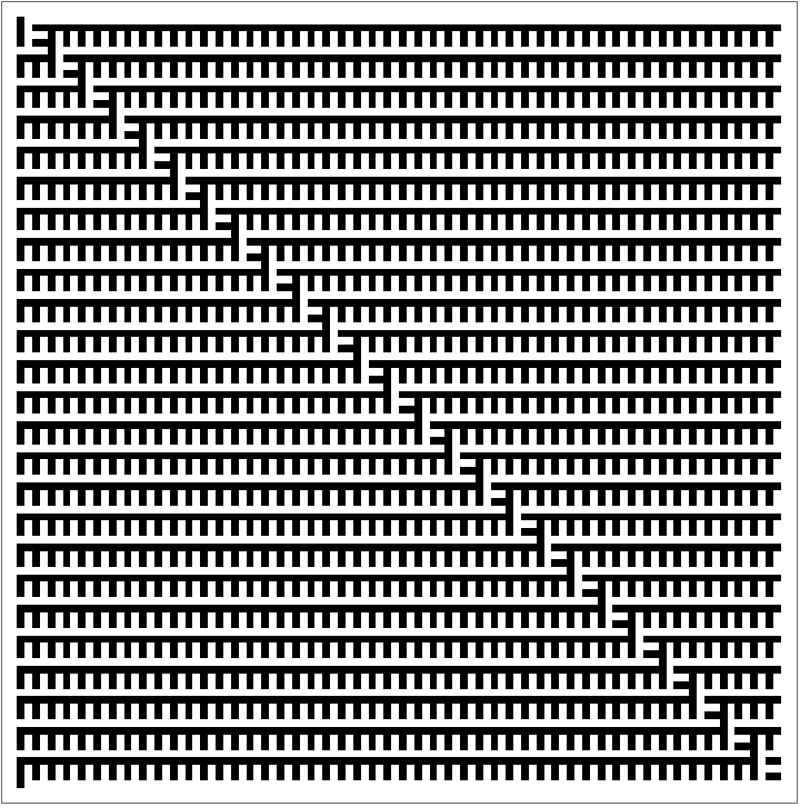
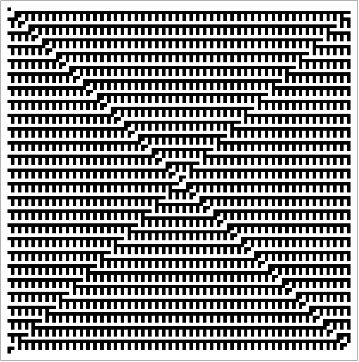
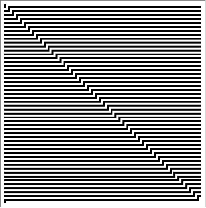
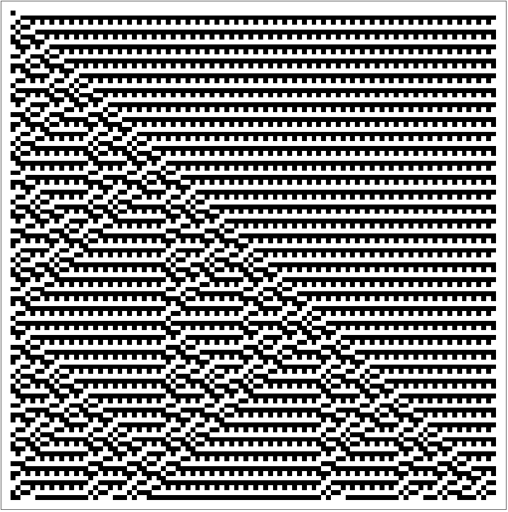
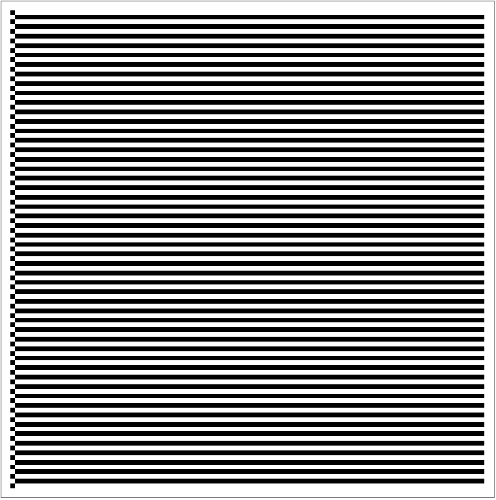
Display all Margolus automata:
However, none of these Margolus rules seem to express much beyond Class 2 behavior, even when using different rules on different clock cycles. When looking for complex behavior in these classical systems, an approach more similar to wolfram ECA seems promising, using 3 channel controlled gates. If any 3 channel gate was used, the gates would not commute past each other and the automaton would need more layers to ensure that the operators in each layer would commute. This can be avoided by limiting the automaton to certain controlled gates. while many quantum operators don't commute, controlled gates which share control lanes can commute past each other.
Controlled operators can overlap control channels and still commute, so these circuits are identical:
To get the desired type of neighborhood 3 automaton, a control structure of 2 controls per gate can be used. If the gate being controlled is arbitrary, these gates can be referred to as CCU gates.
All operators in the same layer can commute past each other:
This can be further generalized to 0-controls, which activate their parent gate with the amplitude of the zero state of the control qubit. These gates can also commute past each other even when the parent gate is sharing the same channel.
Gates on the same channel with different control schemes act independently and therefore commute:
The neighborhood 3 structure can be generalized by iterating over every control structure:
When looking at the classical implementation, it is quite easy to generate all possible automata since the only classical operations which fit into this control structure are NOT and Identity. With four control schemes and two clock cycles, this gives 256 classical automata.
Apply the CCU automaton rule by partitioning the state into overlapping blocks of 3 and applying the respective rule:
Canonicalize these rules and map them to integers to iterate over:
Draw all of the patterns generated by symmetric rules (same operation on even and odd steps):
These symmetric patterns for the CCU automata seem to still be restricted to Class 2 behavior, but certain asymmetric rules do express more complex behavior.
Display all CCU automata:
Some notable CCU automata:
Visualizing Quantum Systems
Visualizing Quantum Systems
The differences of these probabilities are equivalent to the coordinates of the Bloch vector. [4]
In contrast, a mixed state has no certain measurement; this is represented by a vector inside of the Bloch sphere.
Bloch vector of a uniformly mixed state:
Measure along the PauliX, PauliY, and PauliZ directions on a uniformly mixed state:
Now imagine you were to take an entangled Bell Pair and lock the second particle in a box; you only allow yourself to measure the first particle. How would the particle behave?
Measure along the PauliX, PauliY, and PauliZ directions on a single Qubit of a Bell Pair:
The single particle behaves exactly like a perfectly mixed state. Ignoring entanglement between particles, every particle can be mapped to a Bloch vector by measuring in each direction, with maximally entangled particles lying at the center of the Bloch sphere.
Bloch Vectors as Components of the Pauli Basis
Bloch Vectors as Components of the Pauli Basis
While the measurement technique is effective at collapsing entangled states to easier-to-visualize independent Bloch vectors, application of measurement operators in the Wolfram quantum framework is too slow for practical visualization. An alternative solution with linear algebra could offer a substantial speed increase.
A generic single-qubit state:
Measurement probabilities of a generic single-qubit state:
In fact, the Cartesian coordinates of the Bloch vector can be quite easily calculated as expectation values of the Pauli matrices. [5]
Expectation values of the Pauli matrices:
Assuming a pure state, these expectation values are the same as the differences in probabilities above. Using the Kronecker product, this can also be generalized to more qubits.
The Kronecker products of pairs of Pauli matrices form a basis for 4x4 matrices:
PauliX, PauliY, and PauliZ measurement probabilities of the first qubit of the generic state a |00〉+b |01〉+c |10〉+d |11〉:
First qubit Pauli matrix expectation values:
Second qubit probabilities:
Second qubit Pauli matrix expectation values:
The expectation values of the density matrices are equal to the differences in the probabilities so long as the state is normalized. Since the QCA models all start with normalized states and use unitary operators, all of the states in the QCA will also be normalized.
Given a state and an index, find the Bloch sphere coordinates of the qubit at that index, ignoring entanglement:
Some examples of important states we can measure these coordinates for:
These are my desired color assignments for some key points on the Bloch Sphere:
Color function around the shell of the Bloch sphere (Note that SphericalPlot3D normalizes the angles in the color function to 0-1 ranges):
Full Bloch vector color function:
Some examples of color mappings for important states:
Evaluating QCAs
Evaluating QCAs
Given a quantum circuit operator for each clock cycle, the classical CA evaluation function can be quite easily converted to a QCA evaluation function by replacing the classical operations with quantum operations and the classical state with a quantum state. These quantum circuits can be created by iterating over each position and inserting a gate.
Margolus QCA
Margolus QCA
Generate the even clock cycle circuit given the number of qubits (rounded to an even number) and a quantum operator to apply on each pair of qubits:
Generate the odd clock cycle circuit given the number of qubits (rounded to an even number) and a quantum operator to apply on each pair of qubits:
Given a state (row of qubits in the QCA), convert it to a row of colors by the Bloch sphere colorization:
Evaluate the Margolus QCA given the even and odd operations, width, depth, and initial state:
The CX (also known as CNOT) Margolus automaton acting on a basis state is equivalent to a classical Margolus automaton:
When the CX operator spreads a superposition across multiple cells, it becomes an entangled state. Since all of the information in the CA is dependent on the initial state, the whole system is halfway between completely off and the classical automaton evolution.
The CX Margolus automaton on a superposition initial state:
The quantum phase of the initial state is invisible when spread across multiple qubits with this visualization, but when the state recombines to a single qubit, the phase becomes visible again.
The CX operator preserves quantum phase:
The CX Margolus automaton on a larger (10 qubit) system (10 qubits is somewhat close to the limit of what the Quantum Framework paclet can process):
The SWAP Margolus automaton acting on a basis state is also equivalent to a classical Margolus automaton:
The RootSWAP Margolus automaton does not behave classically, instead spreading a definite initial state into a superposition:
The RootSWAP Margolus automaton on a superposition initial state does entangle the qubits, but also maintains a significant pure phase component in each cell:
The phase shifts in each cell are at a relative angle to the initial phase:
A Margolus automaton alternating between CX and SWAP:
A Margolus automaton alternating between CX and RootSWAP:
A Margolus automaton alternating between SWAP and RootSWAP:
CCU QCA
CCU QCA
Unfortunately, I did not get much time to play around with the CCU architecture.
This code should be working, but evaluateCCUQCA has an unknown issue:
Future Goals
Future Goals
The Wolfram Quantum Framework paclet provides helpful and effective tools to evaluate and visualize Quantum Cellular automata. Building off of this work, it would be interesting to see other models implemented with the Wolfram Quantum Framework, in particular the Block-partitioned QCA model [2]. Exploration of models utilizing Fredkin gates may also offer helpful QCA models. Improvements to the evaluation speed of these automata, in particular parallel evaluation of the colorization function, would help with evaluation of larger systems or evaluations of greater depth.
Bibliography
Bibliography
[1] Farrelly, Terry. “A Review of Quantum Cellular Automata.” ArXiv.org, 25 Nov. 2020, https://arxiv.org/abs/1904.13318.
[2] Aoun, Bassam and Tarifi, Mohamad. "Quantum Cellular Automata" ArXiv.org, 20 Jan. 2004, https://arxiv.org/ftp/quant-ph/papers/0401/0401123.pdf.
[3] Perez-Delgado, Carlos A., and Donny Cheung. “Models of Quantum Cellular Automata.” ArXiv.org, 23 Aug. 2005, https://arxiv.org/abs/quant-ph/0508164.
[4] Khrennikov, Andrei. “Quantum-like Representation Algorithm: Transformation of Probabilistic Data into Vectors on Bloch’s Sphere.” ArXiv.org, 10 Mar. 2008, https://arxiv.org/abs/0803.1391.
[6] Schumacher, B., and R. F. Werner. “Reversible Quantum Cellular Automata.” ArXiv.org, 28 May 2004, https://arxiv.org/abs/quant-ph/0405174.
[7] Wagner, Elisabeth, et al. “Information Flow in One-Dimensional Non-Unitary Quantum Cellular Automata.” ArXiv.org, 21 Apr. 2022, https://arxiv.org/abs/2204.09922.
[8] Arrighi, Pablo. “An Overview of Quantum Cellular Automata.” ArXiv.org, 6 Sept. 2019, https://arxiv.org/abs/1904.12956.