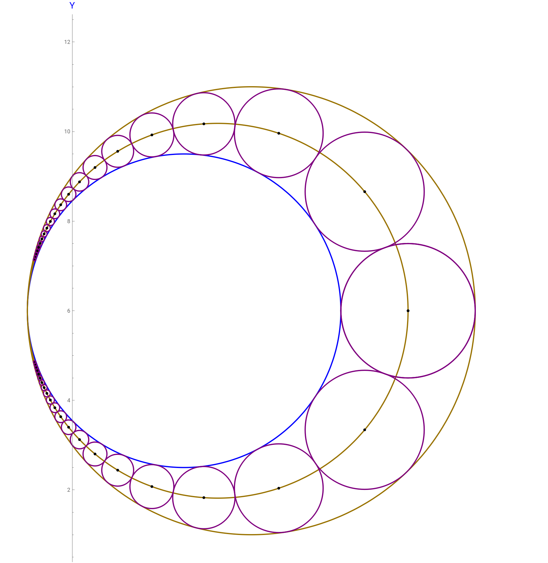
PappusChain::usage="In the Pappus chainwe have in mind the concept of infinity by observing the continuos increase in the number of circumferences (spheres)and the decrease in their size because they occupy a finite space.Reference: Wolfram MathWorld: Pappus chain; Personal"
Animation in 2D:
In[]:=
Manipulater=(7+k1)10;A=-;B=-3-5r;C1=-;D1=-;ShowParametricPlot[{5Cos[θ]+4,5Sin[θ]+6},{θ,0,2π},PlotStyle->{DarkYellow,Thick}],ParametricPlotCos[θ]++,Sin[θ]+6,{θ,0,2π},PlotStyle->{Blue,Thick},ParametricPlotCos[θ]-,Sin[θ]-,{θ,0,2π},PlotStyle->{DarkYellow,Thick},TableGraphicsBlack,PointSize[0.005],Point-1,+r+6,{n,0,20+50k1,1},TableGraphicsBlack,PointSize[0.005],Point-1,-+r+6,{n,0,20+50k1,1},TableGraphicsPurple,Thick,Circle-1,+r+6,,{n,0,20+50k1,1},TableGraphicsPurple,Thick,Circle-1,-+r+6,,{n,0,20+50k1,1},AxesLabel->(Style[#,15,Blue]&/@{"X","Y"}),AxesOrigin{0,0},AxesTrue,BoxedFalse,BoxRatiosAutomatic,ImageSize900,PlotRange{{-1,10},{1,12}},Style["Pappus chain in 2D:",Bold,Medium],Delimiter,{{k1,0,"Value (k1)"},0,3,0.1},ControlPlacementTop
-1-2r-
2
r
4r
3(1+2r+)
2
r
r
-9-14r-4
2
r
r
7+k1
2
5
2
7-(7-k1)
2
7+k1
2
-4AD1+A+
2
B
2
C1
4A
B
2
-4AD1+A+
2
B
2
C1
4
2
A
C1
2A
10r(1+r)
2(+r)
2
n
2
(1-r)
10nr(1-r)
2
n
2
(1-r)
10r(1+r)
2(+r)
2
n
2
(1-r)
10nr(1-r)
2
n
2
(1-r)
10r(1+r)
2(+r)
2
n
2
(1-r)
10nr(1-r)
2
n
2
(1-r)
10(1-r)r
2(+r)
2
n
2
(1-r)
10r(1+r)
2(+r)
2
n
2
(1-r)
10nr(1-r)
2
n
2
(1-r)
10(1-r)r
2(+r)
2
n
2
(1-r)
Out[]=


Animation in 3D:
In[]:=
Manipulater=(7+k1)10;A=-;B=-3-5r;C1=-;D1=-;ShowParametricPlot3D[{5Cos[u]Sin[v]+4,5Sin[u]Sin[v]+6,5Cos[v]+4},{u,0,2π},{v,0,π},PlotStyleDirective[Yellow,Specularity[White,40],Opacity[0.2]],Mesh->None,PerformanceGoal->"Quality",PlotPoints->60],ParametricPlot3DCos[u]Sin[v]++,Sin[u]Sin[v]+6,Cos[v]+4,{u,0,2π},{v,0,π},PlotStyleDirective[Blue,Specularity[White,40],Opacity[0.8]],Mesh->None,PerformanceGoal->"Quality",PlotPoints->60,ParametricPlot3DCos[θ]-,Sin[θ]-,4,{θ,0,2π},PlotStyle->Yellow/.Line[pts_,rest___]:>Tube[pts,0.03,rest],TableGraphics3DBlack,Ball-1,+r+6,4,0.07,{n,0,20+50k1,1},TableGraphics3DBlack,Ball-1,-+r+6,4,0.07,{n,0,20+50k1,1},TableGraphics3DPurple,Specularity[White,40],Opacity[0.5],Sphere-1,+r+6,4,,{n,0,20+50k1,1},TableGraphics3DPurple,Specularity[White,40],Opacity[0.5],Sphere-1,-+r+6,4,,{n,0,20+50k1,1},AxesLabel->(Style[#,15,Blue]&/@{"X","Y","Z"}),AxesOrigin{0,0,0},AxesTrue,BoxedFalse,BoxRatiosAutomatic,ImageSize900,PlotRange{{-2,9},{1,12},{-1,10}},ViewPoint{12,-2.4,10.},Style["Pappus chain in 3D:",Bold,Medium],Delimiter,{{k1,0,"Value (k1)"},0,3,0.1},ControlPlacementTop
-1-2r-
2
r
4r
3(1+2r+)
2
r
r
-9-14r-4
2
r
r
7+k1
2
5
2
7-(7-k1)
2
7+k1
2
7+k1
2
-4AD1+A+
2
B
2
C1
4A
B
2
-4AD1+A+
2
B
2
C1
4
2
A
C1
2A
10r(1+r)
2(+r)
2
n
2
(1-r)
10nr(1-r)
2
n
2
(1-r)
10r(1+r)
2(+r)
2
n
2
(1-r)
10nr(1-r)
2
n
2
(1-r)
10r(1+r)
2(+r)
2
n
2
(1-r)
10nr(1-r)
2
n
2
(1-r)
10(1-r)r
2(+r)
2
n
2
(1-r)
10r(1+r)
2(+r)
2
n
2
(1-r)
10nr(1-r)
2
n
2
(1-r)
10(1-r)r
2(+r)
2
n
2
(1-r)
Out[]=

View of the all angles (below):