Part B: On finding minimal proofs
New tool: “AlphaBetaPrune”
New tool: “AlphaBetaPrune”
Unfortunately, we don’t at present have tools to easily check the recent claim “Othello is Solved”. Our “To Do” list for next year includes an item for obtaining a working reference implementation of AlphaBetaSearch, as a starting place. The paper seems quite difficult, so it will likely need to be checked by an expert in the field. Maybe Andrea will become that expert in five or ten years, who knows.
For now, our analysis of the 4x4 case does not need sophisticated tools. At least one interesting result falls out upon closer analysis. Using the complete Breadth-First-Searched game graph, and the dominance function, we can quickly implement a backtracking algorithm AlphaBetaPrune, which has similar outputs to planned AlphaBetaSearch.
Let’s clarify the distinction between proactive growth algorithms and retroactive pruning algorithms. As a “search” iterates through plausible states, it meanwhile generates directed state-adjacency rules, and eventually grows a graph as output. This is true whether the search is breadth-first or depth-first. We have already seen one example, the entire game graph. When AlphaBetaSearch is implemented, it will ask for a states iterator as input. The usage could be something like this:
AlphaBetaSearch[iterator_,wins_,player_,heuristic_]:=Association["Now"->"More work to be done","Later"->"Outputs a closed subgraph"]
with “wins” assigning values on end conditions, “player” a function for telling whose turn it is, and “heuristic” a function for obtaining a good search order. Once written, this function will depth-first search until it finds a subgraph of the entire game graph, which necessarily is closed under perfect play.
An important fact is that AlphaBetaSearch can only ever find a subgraph of the entire game graph. This fact implies that we can work with a retroactive AlphaBetaPrune, which arrives at similar output by pruning instead of growing. Here is the code for such an algorithm:
In[]:=
AlphaBetaPrune[gg_,dom_,player_,heuristic_:Identity]:=Module[{sort,candidates,state,win,asc,next,res},sort=Association[MapIndexed[#1->#2[[1]]&,heuristic[VertexList[gg]]]];res=DeleteDuplicates[Flatten[Reap[candidates={SortBy[Select[VertexList[gg],VertexInDegree[gg,#]==0&],sort[#]&]};state={candidates[[1,1]]};Sow[state[[1]]];asc=False;While[Length[state]>0,If[And[Not[TrueQ[asc]],SameQ[0,VertexOutDegree[gg,Last[state]]]],asc=True;,If[TrueQ[asc],If[Or[SameQ[Length[Last[candidates]],1],SameQ[player[state[[-2]]],dom[state[[-2]]],dom[state[[-1]]]]],state=Most[state];candidates=Most[candidates];,candidates=ReplacePart[candidates,-1->Rest[candidates[[-1]]]];state=ReplacePart[state,-1->candidates[[-1,1]]];Sow[Last[state]];asc=False;];,next=SortBy[VertexOutComponent[gg,Last[state],{1}],sort[#]&];AppendTo[candidates,next];next=First[next];AppendTo[state,next];Sow[next];];];]][[2]]]];res=Subgraph[gg,res];Graph[res,EdgeList[res]]]
The code is not too bad, but it doesn’t conform to the simple “two while loop” form as seen in many textbook backtracking algorithms. Instead, it’s using an ascending / descending flag “asc”, to switch the per-iteration behavior of the main loop, which terminates on returning to the root vertex. The code is also not too easy, and after one or two failed attempts, we decided to need a quality assurance tool:
In[]:=
TestAlphaBetaConditions[gg_,abg_,dominance_,player_]:=And[AllTrue[Select[VertexList[abg],UnsameQ[dominance[#],player[#]]&],SameQ[VertexOutDegree[abg,#],VertexOutDegree[gg,#]]&],AllTrue[Select[VertexList[abg],SameQ[dominance[#],player[#]]&],Or[VertexOutDegree[abg,#]==0,MemberQ[Lookup[dominance,VertexOutComponent[abg,#,{1}]],dominance[#]]]&]]
Given the entire game graph “gg”, a subgraph “abg”, this function checks closure conditions locally on every vertex. If the current player is not expected to win, the subgraph must expand all possible next moves. If the current player is expected to win, then the subgraph either contains a “next good move” or it has finally reached an end.
Initial exploration
Initial exploration
Our complete solution of 4x4 Reversi is already good enough, but it’s not very easy for a human to understand. With these two additional tools we can now attempt to find a special, particular solution with far fewer nodes. In retrospect, a theorist might have gone about finding “the minimal proof” a different way. As experimentalists, we’re pleased with how well subsequent calculations turned out, and with how much we learned from doing them. Here our discovery of “the minimal proof” is reproduced almost verbatim.
First we take the canonical-reduced game graph, and obtain “player” and “dominance” functions over the nodes of that graph. Respectively these functions determine who plays and who should win:
In[]:=
rgg=;
In[]:=
dominance=Association[ResourceFunction["DirectedAcyclicEvaluate"][ReverseGraph[rgg],Map[#->Sign[Subtract[Length[#[1]],Length[#[2]]]]&,Select[VertexList[rgg],VertexOutDegree[rgg,#]==0&]],Function[If[EvenQ[Length[Last[First[#3]][0]]],Max[#1],Min[#1]]]]["VertexWeights"]];
player=Association[Map[#->Subtract[2Boole[EvenQ[Length[#[0]]]],1]&,VertexList[rgg]]];
Just as a double-check of what we’ve already seen from Andrea, we can plot dominance over the first few levels of the graph:
In[]:=
With[{sg=Subgraph[rgg,VertexOutComponent[rgg,Select[VertexList[rgg],VertexInDegree[rgg,#]==0&],5]]},Graph[sg,GraphLayout->"LayeredDigraphEmbedding",VertexStyle->Map[#->Switch[dominance[#],1,Red,0,LightGray,-1,Blue]&,VertexList[sg]],AspectRatio->1/2,VertexSize->1]]
Out[]=
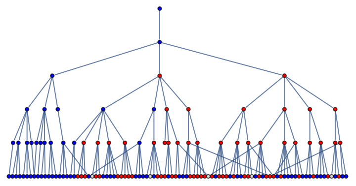
The default of using no heuristic whatsoever leads to a relatively good result:
In[]:=
With[{sg=AlphaBetaPrune[rgg,dominance,player]},test1=Graph[sg,AspectRatio->2/3,VertexSize->1/3,ImageSize->{Automatic,UpTo[400]},GraphLayout->"LayeredDigraphEmbedding",VertexStyle->Map[#->Switch[dominance[#],1,Red,0,LightGray,-1,Blue]&,VertexList[sg]]]]
This graph illustrates an important point: If the initial condition of a game is dominated by one player or another, then a minimal proof of that dominance exists on a subgraph entirely dominated by the expected winner. We have no reason to suspect that 102 vertices is the least possible for a graph satisfying the closure condition, but we can easily do worse:
This particular example seems quite bad, because it takes two wrong turns early on, before finding the winning play in the corner. There are even worse pruning results, according to these statistics:
However, we can improve these statistics by limiting ourselves to the “Beta-dominant” subgraph, which contains only the Beta player’s winning moves:
Pruning from this graph, the statistics become much tighter:
And the minimal vertex count is almost 3 sigma lower than the mean:
Could this possibly be the minimal proof? Before getting our hopes up, let’s try an obvious ordering heuristic, and see if it gets us anything farther:
And indeed, it gets us past 3 sigma, to a graph with only 40 nodes:
Already this is a nice result. If a math party like “Celebration of the Mind” needed entertainment, we could very easily print this out on one page of paper and use it as a cheat-sheet during a work of performance art, perhaps also involving unsuspecting audience members. More to the point, could this possibly be the minimal graph?
At the time of discovery, I conjectured that this 40-vertex proof was minimal, but sadly I also lacked the experience or theoretical insight to complete the proof. Luckily, I had a phone call with Zsombor, explained this problem to him, and he immediately made a suggestion which panned out in the positive. Thanks again, Zsombor, great idea!
Another approach to minimality
Another approach to minimality
Zsombor’s suggestion was just that, perhaps DirectedAcyclicEvaluate could lead trivially to the proof. Hearing this it dawned on me that DAE could probably be used to count vertices, and if so, then that vertex function could be modified with a player-dependent switch. If there’s an easy way to count vertices on a directed acyclic graph, I’ve missed it, and instead will start by converting the beta-dominant subgraph to a tree:
The vertex count function is easy to derive:
The “proof count” function is slightly more difficult. For the winning player it only counts the minimal next branch, while for the losing player it totals all next branches:
The result at the root node is 41, which indicates that our previous result is indeed a minimal result. However, let’s look more closely at the data and check to see if is uniquely minimal:
Blue nodes should not branch, so it looks like there are quite a few viable alternatives. The decision points can be selected easily:
They are all binary choices:
Rather than doing something sophisticated, let’s just check them all by brute force:
And we can also reduce the tree graphs back to directed acyclic form:
Graphs are unique according to their end conditions:
It turns out there 42 different minimal proofs. Here are four of them in entirety:
Up to graph isomorphism, there are only two . One has 8 end conditions, the other has only 7:
This seems to be the most thorough possible answer to our minimality question.
This was a nice example. Thanks again, Andrea, for suggesting it!