Double Pendulum is the simplest mechanical system without friction and external forcing that demonstrates chaos. Integrable systems (none-chaotic) require the number of independent conserved quantities to match the number of degrees of freedom. The simple pendulum meets this criterion, whereas the double pendulum does not, resulting in its non-integrable and chaotic nature. Double pendulum has 2 degrees of freedom (2 angles) and just 1 conserved quantity (total mechanical energy).
To observe chaos double pendulum we can build different visualizations. But there is one I highly enjoy -- it is many double pendulums for various initial conditions by Jonathan Nafziger. I want to recreate it with Wolfram Language.
In Wolfram ecosystem we have quite a few examples of double pendulum:
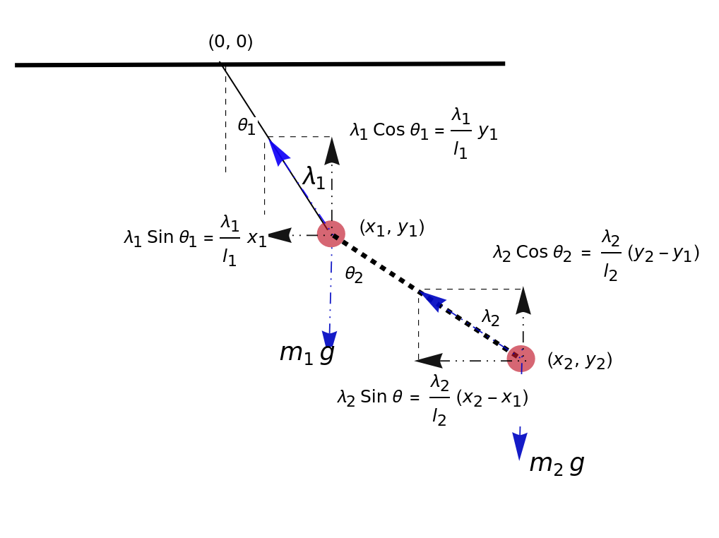
Start by defining a function to depict a single double pendulum with simple two lines:
In[]:=
ClearAll[douBpenD]douBpenD[angle1_,angle2_,radius1_,radius2_,{x0_,y0_}]:= Module[{x1,y1,x2,y2}, x1=x0+radius1 Sin[angle1]; y1=y0-radius1 Cos[angle1]; x2=x1+radius2 Sin[angle2]; y2=y1-radius2 Cos[angle2]; Graphics[{Opacity[.9],Line[{{x0,y0},{x1,y1}}],Line[{{x1,y1},{x2,y2}}]}] ]douBpenD[Pi/4,-Pi/4,1,1,{0,0}]
Out[]=
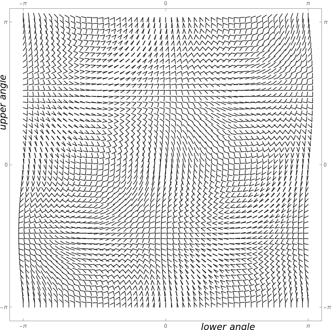
The next function places 2500 double pendulums on 50x50 grid where each spot corresponds to a different initial angles values:
In[]:=
ClearAll[viz]viz[tbl_]:=Column[{Style["2,500 Double Pendulums",25,Opacity[.8],Darker@Red,FontFamily->"Copperplate"],Style["Varying Initial Angles: Domains of Chaos and Order",17,Opacity[.7],Darker@Red,FontFamily->"Georgia"],Show[tbl,PlotRange->Pi,PlotRangePadding->.3,Frame->True,BaseStyle->15,ImageSize->540,FrameTicks->{Range[-Pi,Pi,Pi],Range[-Pi,Pi,Pi]},Epilog->{Inset[Style["lower angle",Italic],Scaled[{.7,-.02}]],Inset[Rotate[Style["upper angle",Italic],Pi/2],Scaled[{-.02,.7}]]}]},Alignment->Center]viz@Flatten[Table[douBpenD[a1,a2,.1,.1,{a2,a1}],{a1,-Pi,Pi,Pi/25},{a2,-Pi,Pi,Pi/25}]]
Out[]=
2,500 Double Pendulums |
Varying Initial Angles: Domains of Chaos and Order |
A single function from Wolfram Function Repository solves numerically the double pendulum:
In[]:=
ResourceFunction["DoublePendulumFormula"]
Out[]=
Using it we compute evolution of all 2500 double pendulums for 10 seconds:
In[]:=
n=50;evo=ParallelTable[Association["l1"->1,"l2"->1,"m1"->1,"m2"->1],Association["theta1i"->a1,"theta2i"->a2,"t"->10]],{a1,-Pi,Pi,2Pi/(n-1)},{a2,-Pi,Pi,2Pi/(n-1)};//AbsoluteTiming
Out[]=
{6.20134,Null}
In[]:=
evo//Dimensions
Out[]=
{50,50}
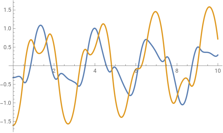
Here is angles evolution of a sample single double pendulum from our grid:
In[]:=
Plot[{evo[[23,13]]["Angle1Solution"][t],evo[[23,13]]["Angle2Solution"][t]},{t,0,10}]
Out[]=
And this is how this double pendulum looks at t=4:
In[]:=
douBpenD[evo[[23,13]]["Angle1Solution"][4],evo[[23,13]]["Angle2Solution"][4],1,1,{0,0}]
Out[]=
Compute the range of 50 angles along single angle axis to use as initial conditions:
In[]:=
rg=Range[-Pi,Pi,2Pi/(n-1)]
Out[]=
-π,-,-,-,-,-,-,-,-,-,-,-,-,-,-,-,-,-,-,-,-,-,-,-,-,,,,,,,,,,,,,,,,,,,,,,,,,π
47π
49
45π
49
43π
49
41π
49
39π
49
37π
49
5π
7
33π
49
31π
49
29π
49
27π
49
25π
49
23π
49
3π
7
19π
49
17π
49
15π
49
13π
49
11π
49
9π
49
π
7
5π
49
3π
49
π
49
π
49
3π
49
5π
49
π
7
9π
49
11π
49
13π
49
15π
49
17π
49
19π
49
3π
7
23π
49
25π
49
27π
49
29π
49
31π
49
33π
49
5π
7
37π
49
39π
49
41π
49
43π
49
45π
49
47π
49
Manipulate will show full 10 seconds evolution of all 2500 double pendulums:
In[]:=
Manipulate[viz[Flatten[Table[douBpenD[evo[[x,y]]["Angle2Solution"][t],evo[[x,y]]["Angle1Solution"][t],.1,.1,{rg[[x]],rg[[y]]}],{x,1,n},{y,1,n}]]],{t,0,10}]
Compute 300 rasterized frames:
And make a video:
CITE THIS NOTEBOOK
CITE THIS NOTEBOOK
2500 double pendulums. Varying initial angles: domains of chaos and order.
by Vitaliy Kaurov
Wolfram Community, STAFF PICKS, November 26, 2024
https://community.wolfram.com/groups/-/m/t/3328657
by Vitaliy Kaurov
Wolfram Community, STAFF PICKS, November 26, 2024
https://community.wolfram.com/groups/-/m/t/3328657