Fitness-neutral sets are observed in systems where genotype-phenotype mapping displays a many-to-one relationship. This study highlights the phenomena of percolation where multiple genotype specimens which manifest a single phenotype originate from diverse areas of configuration space. We show that percolation is a probable feature of certain scenarios in Stephen Wolfram’s minimal model for biological evolution and argue that the production of percolating fitness-neutral sets and the analysis thereof can be of use in biological studies and possibly in other relevant scientific areas.
Fitness-Neutral Sets and Percolation
Fitness-Neutral Sets and Percolation
What is a fitness-neutral set?
What is a fitness-neutral set?
In some systems a chain of genotype specimens whose adjacent members are connected to each other by subsequent single-point mutations maps in its entirety a single phenotype. Such a chain is called a fitness-neutral set. In Stephen Wolfram's minimal model for biological evolution [1], a fitness-neutral set is a chain of cellular automata rules (the genotype) that map, for example, to a single lifetime (the phenotype). In RNA research, a fitness-neutral set is known as a neutral network (both terms will be interchangeably used in this essay), and is a chain of RNA sequences that map to a single RNA secondary structure.
What is percolation?
What is percolation?
Do fitness-neutral sets span the entire configuration space or are they limited to small islands therein? Percolation alludes to the former observation. Schuster, Fontana, Stadler and Hofacker [2] showed that RNA sequences forming neutral networks percolate in sequence space and cited the strong implications it has on the underlying system (e.g., epistasis). Reidys, Stadler and Schuster [3] put forth a scheme of quantifying RNA neutral networks that included criteria for percolation.
Percolation: fundamental metrics and major criteria
Percolation: fundamental metrics and major criteria
In this work we used two neutral networks metrics:Average Local Neutrality - the mean of phenotype-conserving single-point mutations across members of a neutral network.Network Diameter - the maximum Hamming distance between any two members of the neutral network. And two percolation criteria imposed on them:1. Average local neutrality of the neutral network, λ, is larger than λ* = where α = alphabet size, e.g. α=4 for RNA sequences and α=3 for (k=3, r=1) CA rule space.2. If a neutral network percolates then 𝔇, the diameter of the subgraph connecting its nodes, is larger than 𝔇* = Diameter of configuration space, e.g. 𝔇*=64 for RNA sequences and 𝔇*=27 for (k=3, r=1) CA rule space. The reverse is not necessarily correct and requires proof, herein we will provide a demonstration to this direction rather than a sound proof.
α-1
1
α
A Few Words on the Code
A Few Words on the Code
Most of the code in this notebook was developed with the help of the Wolfram Notebook Assistant. Cellular automata and graphic inline functions were provided to me by my mentor Willem Nielsen.
Before we start, a few functions need to be evaluated in order for the rest of the code in the notebook to work.
Before we start, a few functions need to be evaluated in order for the rest of the code in the notebook to work.
Evaluate the (collapsed) input cell below:
Code
Code
Cellular Automata Rules and Average Local Neutrality
Cellular Automata Rules and Average Local Neutrality
In this study, we limited ourselves to computational experiments on the (k=3, r=1) cellular automata rule space and to adaptive evolution simulations starting from a default initial condition.
Consider a cellular automata rule in (k=3, r=1) with a default initial condition and lifetime of 1:
In[]:=
ArrayPlot[CellularAutomaton[{3818007614403,3,1},{{0,0,0,0,0,1,0,0,0,0,0},0},{1,11}],ColorRules->{0->White,1->Orange,2->Blue},Mesh->True]
Out[]=
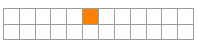
Let us examine the rule bits:
In[]:=
ArrayPlot[{IntegerDigits[3818007614403,3,27]},ColorRules->{0->White,1->Orange,2->Blue},Mesh->True]
Out[]=

In order for the rule to have a lifetime of 1 with a default initial condition all that is required are the 18th, 24th, 26th and 27th rule bits to be set to zero, since these correspond to the four relevant neighbourhoods in the initial condition, {1,0,0}, {0,1,0},{0,0,1} and {0,0,0} respectively. Any (k=3, r=1) rule with these four bits set to zero has a lifetime of 1.
That means that out of the 52 available single-point mutations (the null rule being a fixed point), such rule always has 46 neutral ones. This poses a high value for its local neutrality (46/52=0.88). And this fact sets up a high probability for the formation of large fitness-neutral sets of rules with an average local neutrality of 0.88 which is far higher than λ* for the (k=3, r=1) rule space which equals 0.58.
That means that out of the 52 available single-point mutations (the null rule being a fixed point), such rule always has 46 neutral ones. This poses a high value for its local neutrality (46/52=0.88). And this fact sets up a high probability for the formation of large fitness-neutral sets of rules with an average local neutrality of 0.88 which is far higher than λ* for the (k=3, r=1) rule space which equals 0.58.
Let us demonstrate the above for clarity:
In[]:=
FitnessRayPlot[{3818007614403,3,1},(TestLifetime[#,100]&)]
Out[]=
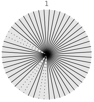
In this case the six non-neutral single-point mutation diverge to a practically infinite lifetime (denoted by dotted lines) which guarantees the continuity of the fitness-neutral set in an adaptive mutation process. In fact, such is a property of over 90% of lifetime 1 rules, which promotes the formation of large fitness-neutral sets.
Try out a to evaluate the below code a few times to get a feel of the frequency at which the initial four white bits change (the rightmost can never change):
In[]:=
tenWalk=[<|"AdaptiveIterations"->10,"InitialRule"->{3818007614403,3,1},"MaxSteps"->120|>,"RuleChanges",{"BestRule"}][[All,1]];RulesMutationPlot[tenWalk,"GapSize"->3]
Out[]=
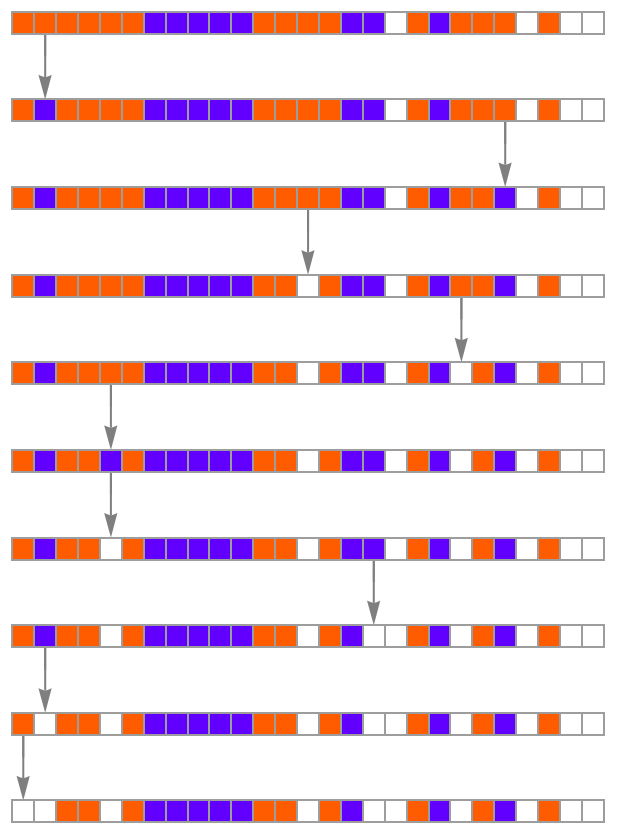
Thus, in the scenario described above the minimal model for biological evolution features the formation of fitness-neutral sets which meet the average local neutrality criteria for percolation.
Adaptive Evolution and Average Local Neutrality
Adaptive Evolution and Average Local Neutrality
At this point, we can devise a methodology by which to test the second percolation criteria regarding network diameter and also examine what happens after the fitness-neutral sets of lifetime 1 find the “porthole” through which they escape to higher lifetimes.
The chosen methodology is random walks starting from a rule with a lifetime of 1 over which an adaptive evolution simulation is performed by the resource function AdaptiveCellularAutomaton for a user-defined number of iterations.
The chosen methodology is random walks starting from a rule with a lifetime of 1 over which an adaptive evolution simulation is performed by the resource function AdaptiveCellularAutomaton for a user-defined number of iterations.
Adaptive mutation simulation - walkthrough
Adaptive mutation simulation - walkthrough
Pick a random rule and apply AdaptiveCellularAutomaton:
In[]:=
SeedRandom[19670809];ruleWithLifetime1K3R1=Join[Flatten[{searchForLifetimeOneRules[1]}],{3,1}];numIterations=2500;rules=[<|"AdaptiveIterations"->numIterations-1,"InitialRule"->ruleWithLifetime1K3R1,"MaxSteps"->120|>,"RuleChanges",{"BestRule","BestFitness","Index"}];gatheredRules=GatherBy[rules,#BestFitness&];
Process and output run results:
In[]:=
lifetimeChangeData=analyseMutations[gatheredRules];createLifetimeTable[rules,numIterations,lifetimeChangeData]
Out[]//TableForm=
# | Lifetime | Iterations | Diameter | Norm_Diam | Cum_Neut_Prob | Avg_Loc_Neut |
1 | 1 | 613 | 541 | 0.88 | 0.79 | 0.88 |
2 | 2 | 93 | 86 | 0.94 | 0.12 | 0.78 |
3 | 3 | 14 | 12 | 0.93 | 0.68 | 0.73 |
4 | 4 | 12 | 11 | 1.00 | 0.63 | 0.65 |
5 | 5 | 26 | 21 | 0.85 | 0.48 | 0.51 |
6 | 7 | 28 | 26 | 0.96 | 0.42 | 0.52 |
7 | 11 | 8 | 7 | 1.00 | 0.22 | 0.26 |
8 | 21 | 5 | 4 | 1.00 | 0.05 | 0.15 |
9 | 26 | 2 | 1 | 1.00 | 0.29 | 0.09 |
10 | 34 | 3 | 2 | 1.00 | 0.30 | 0.08 |
11 | 59 | 3 | 2 | 1.00 | 0.19 | 0.08 |
12 | 99 | 9 | 2 | 0.33 | 1.00 | 0.08 |
Active Mutations | 816 | |||||
Number of Iterations | 2500 | |||||
Run Efficacy | 0.57 |
A lot can be learned from these results:
■ The large neutral network of lifetime 1 which meets both percolation criteria (λ > λ*=0.58, 𝔇 > 𝔇*=27).
■ Lifetime 2 also meets both percolation criteria.
■ Average local neutrality decreases as lifetime increases resulting in smaller, non-percolating neutral networks.
■ Run efficacy measures the amount of idle iterations - with low efficacies, such as 0.57, a high number of lifetime hops is expected throughout the simulation.
■ In this example the simulation could not reach 2500 iterations because none of the lifetime 99 mutations resulted in a finite increase in lifetime. This can also be seen from the cumulative neutrality probability value of lifetime 99 which is 1, i.e. the adaptive process accepted nine lifetime conserving mutations and halted thereafter.
Adaptive Evolution and Percolation
Adaptive Evolution and Percolation
Evidence of percolation
Evidence of percolation
Thus far in this example we saw a strong indication to the existence of percolating fitness-neutral sets for two lifetimes (1 and 2).
However, as mentioned before, meeting the diameter criteria is not enough: a percolating fitness-neutral set will satisfy 𝔇 > 𝔇*=27 however not every fitness-neutral set that satisfies 𝔇 > 𝔇*=27 is percolating. There can exist such sets that expand in the (k=3, r=1) 27D hypercube yet occupy a small portion of space therein, such sets are said to exhibit a “snake-like” structure.
In the original essay we provided the two indications below that the case of adaptive evolution simulations of the fitness-neutral sets under our lamp seems to be one of percolation.
In the addendum we provide a better and more convincing visualization for that.
3D visualization of the fitness-neutral set
3D visualization of the fitness-neutral set
If a fitness-neutral set is percolating we expect a dimension-reduced plot of it to be non-compact. Admittedly, this is a weaker intuition-driven indication since a 27D space is hard to grasp and also its reduction to 3D. Yet we feel it is interesting to put it on display.
Dimension-reduction for the 3D plot of the fitness-neutral set with lifetime 1 from the adaptive evolution simulation above (collapsed code):
In[]:=
(*3Dreduced-dimensionplotforlifetime=1only*)ruleNumbersRw=gatheredRules[[1]][[All,1,1]];(*Converteachdecimalnumbertoa27-digitbase3string*)base3Numbers=IntegerString[#,3,27]&/@ruleNumbersRw;(*Functiontoconvertbase-3stringsto3Dcoordinates*)to3DCoordinates[str_]:=Module[{digits},digits=ToExpression[Characters[str]];{Total[digits[[1;;9]]],Total[digits[[10;;18]]],Total[digits[[19;;27]]]}];(*Converteachbase-3stringto3Dcoordinates*)coordinates=to3DCoordinates/@base3Numbers;(*Createlinesbasedonadjacencyinthelist*)lines=Line/@Partition[coordinates,2,1];(*Visualizethegraphin3Dwithsmallspheres*)Graphics3D[{{Sphere[#1,0.1]&/@coordinates},{Thick,lines}},Boxed->False,ImageSize->Large]
Random walk, quasi-random walk and non-random walk
Random walk, quasi-random walk and non-random walk
Apart from the random walk we demonstrated we deployed two more: a non-random walk where fitness-neutral sets are “harvested” from the multiway graph of (k=3, r=1) with a breadth-first search approach, and a quasi-random walk where we still “harvest” the multiway graph yet allow random depth passages farther away in it.
‘A convex hull is the smallest convex shape that encloses a set of points in a geometric space. It can be visualized as the shape formed by stretching a rubber band around the outermost points of the set. In computational geometry, the convex hull is commonly used to simplify complex shapes and to analyze spatial properties such as the area or boundary of a dataset.’ (Wolfram Notebook Assistant)
After constructing these three fitness-neutral sets, we use ConvexHullMesh over a dimension reduction to 2D to estimate the “area” of the random, quasi-random and non-random fitness-neutral sets all starting from the same lifetime 1 rule.
Formation of quasi-random and non-random walks and calculation of convex hull area (collapsed code):
Note: evaluation of the second cell is time-consuming.
Note: evaluation of the second cell is time-consuming.
Albeit a work-in-progress, in most adaptive evolution simulations we performed thus far data and plots demonstrate that random walks expectedly have a striking advantage in diameter and an advantage in (normalized) projected area.
Evaluate (collapsed) cell below to display data:
Random walk, quasi-random walk and non-random walk - sample graphs
Random walk, quasi-random walk and non-random walk - sample graphs
Random walk 2D graph
Quasi-random walk 2D graph
Non-random walk 2D graph
Addendum: further evidence of percolation using the random, quasi-random and non-random concept
Addendum: further evidence of percolation using the random, quasi-random and non-random concept
We consider two more geometric metrics that can provide further evidence for percolation-like pattern of a set of points scattered in a hypercube:
Radius of Gyration - the root mean squared Hamming distance of points from their centroid, quantifies the spacial extent of the set.
Average Inter-point Distance - the mean Hamming distance between any pair of set members, measures the overall dispersion of the set in configuration space.
As the radius of gyration approaches its maximal Hamming diameter, 27 in our case, the set increasingly traverses the hypercube. Similarly, as the average inter-point distance (also known as sparsity) approaches its maximal value, 18/27 ≈ 0.66 in our case, the diversity of the set increases.
Taken together, these metrics can provide evidence for expansion of a fitness-neutral set in hyperspace while disfavoring narrow, snake-like propagation.
Let us examine an adaptive evolution simulation:
This simulation creates a random walk fitness-neutral set of lifetime 1 of size 317 and diameter 280, a quasi-random walk of size 1370 and diameter 14 and a non-random walk of size 1059 and diameter 4.
Calculating and displaying the two metrics for the above sets, it is seen that despite it is the smallest set by far the random walk traverses hyperspace
the most and is the most diverse. The quasi-random walk catches up on the random walk only on radius. Expectedly, the non-random walk lags behind considerably.
Concluding Remarks
Concluding Remarks
This study claims that random adaptive evolution walks on a default initial condition on (k=3, r=1) seem to produce percolating fitness-neutral sets for lower lifetime values (especially 1). Much of it was done on the fly and at a high pace, yet we feel its results are a stepping stone to further experiments. Implications of variable initial conditions need to be considered. More concise ways to measure distribution in 27D should be learned and implemented. Should we draw closer to the RNA case, the relevant rule space seems to be (k=4, r=2) which is dozens of orders of magnitude bigger than (k=3, r=1) posing computational challenges of a new level. More data from more executions of the adaptive evolution framework that is decided should be accumulated and processed.
On a personal note, i found the new way in which to do science extremely plausible. Trying to minimize the glass ceiling imposed by computational irreducibility by intuition that directed me towards making the “correct computations” (an ever-changing term) seems to be the best way to gain insight into the complex systems under research, where it seems that the rigorous tools of olden times are becoming less efficient.
On a personal note, i found the new way in which to do science extremely plausible. Trying to minimize the glass ceiling imposed by computational irreducibility by intuition that directed me towards making the “correct computations” (an ever-changing term) seems to be the best way to gain insight into the complex systems under research, where it seems that the rigorous tools of olden times are becoming less efficient.
Acknowledgments
Acknowledgments
I would like to thank my mentor Willem Nielsen for sharing his vast Wolfram Language knowledge with me and for challenging discussions which helped this computational study take shape. Thanks to Willem this Winter School was a highly exciting learning experience for me. I am also extending my gratitude to Stephen Wolfram for reshaping my initial thoughts on this study and directing it to new thought-provoking areas and to a first-time deployment of a new scientific thought process.
References
References
◼ [1] Wolfram (2025), “Why Does Biological Evolution Work? A Minimal Model for Biological Evolution and Other Adaptive Processes”, Complex Systems, 33(4), 387-488. https://doi.org/10.25088/ComplexSystems.33.4.387
◼ [2] Schuster, Fontana, Stadler and Hofacker (1994), “From Sequences to Shapes and Back: A Case Study in RNA Secondary Structures”, Proceedings of the Royal Society of London B (Biological Sciences), 255, 279-284. https://doi.org/10.1098/rspb.1994.0040
◼ [3] Reidys, Stadler and Schuster (1997), “Generic properties of combinatory maps: Neutral networks of RNA secondary structures”, Bulletin of Mathematical Biology, 59 (2), 339-397. https://doi.org/10.1007/BF02462007
CITE THIS NOTEBOOK
CITE THIS NOTEBOOK
Percolation in fitness-neutral sets in the minimal model for biological evolution
by Rami Zakh
Wolfram Community, STAFF PICKS, January 15, 2026
https://community.wolfram.com/groups/-/m/t/3607149
by Rami Zakh
Wolfram Community, STAFF PICKS, January 15, 2026
https://community.wolfram.com/groups/-/m/t/3607149