This project first explores the use of SK combinators to perform arithmetic operations on Church numerals. The project determines their size and time complexity and verifies their optimality through various ways. Several efficient combinators are also found. The project then proposes a new method to construct SK combinators for binary representations of arbitrary length efficiently and bitwise operations. At the end, the project compares their efficiency and the performance to do basic arithmetic.
Introduction
Introduction
SKI and SK Combinators
SKI and SK Combinators
The SKI combinator calculus is a computational system that was introduced by Moses Schönfinkel and Haskell Curry in the early 20th century (SKI Combinator Calculus). It is important in the study of theoretical computer science as it is proven to be Turing complete, meaning it can perform any calculation with unlimited time and memory. The SKI combinator calculus is made of three combinators, S, K, and I, that can be defined in lambda expressions as follows:
S = λx.λy.λz.xz(yz) K = λx.λy.x I = λx.x
The S combinator takes three parameters and applies the first two to the third. The K combinator takes two parameters and returns only its first. The I combinator returns the only parameter itself.
The SK combinator calculus, on the other hand, is a reduced version of the SKI combinator calculus, where it is proven that the I combinator can be represented in only S and K combinators, meaning that S and K combinators are a minimal complete set and they can represent any lambda expression. It is a programming language with only two letters. Here is how it works:
S K K x = K x (K x) = x = I x I = S K K
Combinators S and K are two built in symbols in the Wolfram Language:
In[]:=
CombinatorS
Out[]=
S
In[]:=
CombinatorK
Out[]=
K
In the Wolfram Language, we can evaluate an SK combinator by repeatedly replacing S and K combinators with their rules.
Functions to evaluate SK combinators:
In[]:=
combinatorRules = {CombinatorS[x_][y_][z_] x[z][y[z]], CombinatorK[x_][y_] x};combinatorEvaluate[f_] := f //. combinatorRulescombinatorReplace[f_] := f /. combinatorRules
The function combinatorReplace is to replace rules by only once, whereas the function combinatorEvaluate will keep replacing rules until reach the fix point.
An example for the combinator I that is represented in terms of SK combinators:
In[]:=
combinatorEvaluate[S[K][K][x]]
Out[]=
x
To convert a lambda expression to SK combinators, the resource function SKCombinatorCompile can be used:
Function to compile a combinator:
In[]:=
combinatorCompile[arg_, f_] := ResourceFunction["SKCombinatorCompile"][f, arg]
The first parameter includes a list of parameters, and the second parameter is the body part of the lambda expression.
Examples:
λa.λb.λc.c (a b)
In[]:=
combinatorCompile[{a,b,c},c[a[b]]]
Out[]=
S[K[S[K[S[S[K][K]]]]]][S[K[K]]]
λa.λb.λc.c (a (λd d c b))
In[]:=
combinatorCompile[{a,b,c},c[a[combinatorCompile[{d},d[c][b]]]]]
Out[]=
S[K[S[K[S[S[K][K]]]]]][S[S[K[S]][S[K[K]][S[K[S]][K]]]][K[S[K[S[S[K[S]][S[K[S[S[K][K]]]][K]]]]][S[K[K]][K]]]]]
Church Numerals
Church Numerals
Church numerals are representations of natural numbers using lambda notation. The function that represents the Church numeral of any natural number applies a function to an initial values times as follows:
n
f
x
n

For example:

In the Wolfram Language, we can nestedly apply a function f to a value x by using the function Nest:
In[]:=
Nest[f,x,5]
Out[]=
f[f[f[f[f[x]]]]]
Functions to convert an integer to a church numeral and to convert it back:
In[]:=
intToChurch[n_] := Nest[successor, zero, n]churchToInt[f_] := Depth[f]-1
The definition of successor and zero, which are also represented by SK combinators, will be elaborated later in the section of Previous Works.
The Church numeral serves as a common way to represent natural numbers in lambda calculus, as well as SK combinator calculus. However, it has constraints of being difficult to perform bitwise operations because getting each of its digits in binary is largely inefficient since it involves division and modulus. However, a binary number system might be a more efficient numeral system to perform bitwise operations.
Binary Number System
Binary Number System
Binary Representation
Binary Representation
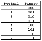
All computations by our computers are done in the binary number system. It is a numeral system that is expressed in the base of 2, such that each digit is eighter 1 or 0. Binary numbers of n digits can represent different numbers from to -1. For example, numbers in decimal, which are in the base of 10, can be converted to binary numbers of 3 digits as follows:
n
2
0
n
2
Binary Conversion
Binary Conversion
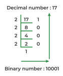
To convert a decimal number to the binary form, we need to get the value of each of its digits from the first digit (the right most digit) in the binary form. The first digit is the value of the decimal number mod 2. To get following digits, we need to divide the number by 2 and only keep the integer part. We do the same steps until the decimal number equals zero. For example:
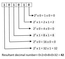
To convert a binary number back to the decimal form, we only need to sum up the of each digit that is 1, where i its a zero index for its digit from the right most. For example:
i
2
Bitwise operations can be easy to perform in a binary number system because it is mainly about the values of each digit in binary. Several bitwise operations are and, or, xor, nand, and so on. It is proven that nand is a minimal complete set, which can represent any bitwise operation.
Previous works
Previous works
Church Numerals, Successor, and Zero
Church Numerals, Successor, and Zero
SK Combinators for Arithmetic Operations
SK Combinators for Arithmetic Operations
Boolean SK Combinators
Boolean SK Combinators
The reason we need SK combinators for Boolean logic is to perform some conditional logic computations by using SK combinators. To build these logic operations, we need to first define the two most important logic units, true and false in SK combinators. We usually use true and false in an if statement, such as:
In[]:=
If[True,a,b]
Out[]=
a
and
In[]:=
If[False,a,b]
Out[]=
b
The use of true will always take the first value, whereas false takes the second.
Let’s define the lambda expression for the function if, first, and second to be:
if = λp.λa.λb.p a b first = λa.λb.a second = λa.λb.b
According to the lambda expressions, we then can get their SK combinators through compiling:
In[]:=
if=combinatorCompile[{p,a,b},p[a][b]]first=combinatorCompile[{a,b},a]second=combinatorCompile[{a,b},b]
Out[]=
S[K][K]
Their shortest SK combinators:
Note that you can understand First as True, and Second as False.
Stephen Wolfram has found the minimal SK combinators for all bitwise operations of length up to one by search (Wolfram):
In addition to finding these SK combinators for bitwise operations of length of one through search, we can also construct them by compiling.
Compile the SK combinator for the xor operation of length of one:
This expression is like a nested if statement where if both parameters are true or both of them are false, which goes to either the first or the fourth case, it returns false, otherwise it returns true.
Simplify the combinator by replacing b[true][false] with b:
For example, this code returns the combinator K, which stands for the false:
We can utilize the idea to construct binary representation by first constructing its logic units true and false and this way to compile through nested if statement in the later part of this essay to construct the binary representation of any length.
Finding Optimal Combinator Representations for Arithmetic
Finding Optimal Combinator Representations for Arithmetic
My initial research question was finding optimal combinator representations for arithmetic (addition, multiplication, and exponentiation) with different ways to represent integers. However, I was able to verify through brute force that Wolfram’s expressions are already minimal much quicker than expected, and expressions for arithmetic operations are independent of the successor function (will later be elaborated). However, I still found several other efficient combinator representations for arithmetic.
We can find other SK combinators that can also do these arithmetic operations through different ways.
Before starting, to test the optimality of a combinator, we need to take views from two aspects, its size and its number of steps to the fix points. Usually, the smallest the size, the less steps to the fix point; however, this is not always true. That is why we need to try different methods rather than just brute force.
Functions to return the size of a combinator and the number of steps to its fixed point
Direct Compiling
Direct Compiling
Let’s first try to directly compile each of arithmetic operations
Addition
Addition
Given that the lambda expression for addition is:
Compile its combinator according to the lambda expression:
This plus combinator has a size of 10, which is one unit longer than the one in Stephen Wolfram’s book.
Multiplication
Multiplication
The lambda expression for multiplication is:
Compile its combinator according to the lambda expression:
Simplify the expression:
It gives the same SK combinator as the one Stephen Wolfram found in his book.
Exponentiation
Exponentiation
The lambda expression for exponentiation is:
Compile its combinator according to the lambda expression
Simplify the expression
It also gives the same SK combinator as the one Stephen Wolfram found in his book.
Brute Force Enumeration
Brute Force Enumeration
We can brute forcibly enumerate all SK combinators smaller than or equal to the size of each arithmetic SK combinator to verify the optimality of the current ones.
We can generate all combinations of SK combinators of a given size n through recursion:
Here, I applied the DFS memorization so that for each n, find[n] will only be computed at most once, largely speed up the code.
Or, you can enumerate combinators by the resource function EnumerateCombinators:
Building a graph for the relationships between combinators, we create a directed edge if one combinator can transfer to another by applying the rules once. Since one combinator can transfer to different combinators by changing the order of applying rules, and the multiple different combinators can lead to a same final expression or the fix point, the relationship between combinators is a DAG graph (directed acyclic graph) rather than a tree. For any two combinators, if they are connected by a road or path, they are equivalent, and for any combinator, there are infinite equivalent combinators as you can keep replacing the rule of combinator K on it. In some rare cases, their relationships aren’t a DAG graph but can form cycle. In this situation, the combinator has no fixed point and its evaluation will never halt.
Function to find SK combinators equivalent to a given lambda expression:
This function deletes equivalent combinators, such one that is another’s ancestor (lead to a same combinator during the evaluation process). To avoid infinite evaluation, we set the parameter steps to perform a fix number of replacement; however, this might miss some potential combinators that also work.
Since the number of SK combinators increases exponentially, we only want to check combinators of size 9 or less.
Addition
Addition
The current minimal addition combinator has a size of 9. Let’s enumerate all SK combinator with the size of 9 or less.
It is shown that the only SK combinator with size 9 or less is the one Stephen Wolfram found, showcasing its minimality.
Multiplication
Multiplication
Within the size of 5, there is only one combinator for multiplication, showing its minimality.
However, within the range of 6, there are 17 combinators for multiplication.
It’s interesting to consider how will the number of combinators will grow as the size get bigger.
Visualize the distribution of combinators for multiplication:
The number of combinators for multiplication increases exponentially as the size increases. An exception happens at the size of 4 to 5, which decreases a bit.
Exponentiation
Exponentiation
The current minimal exponentiation combinator has a size of 7. Let’s enumerate all SK combinator with the size of 7 or less.
There are four combinators of size 7 for exponentiation. Let’s compare their efficiency to the fixed point:
It is found that there exists another combinator for exponentiation of the same size and efficiency.
Visualize the distribution of combinators for multiplication
The number of exponentiation combinators increases dramatically when the size is 8 to 9.
Compiling Addition from Successor
Compiling Addition from Successor
Finding smaller combinators through enumeration shows that the current one is already minimal with the lambda expression for addition. I tried to compile addition with an alternative lambda expression for addition that is based on successor, which I hope can find shorter combinators in this way.
Addition’s Successor-based Lambda Expression
Addition’s Successor-based Lambda Expression
The nature of addition is to apply successor a number of times to a number. For example, 2+3 means to apply successor to 3 twice. We can therefore have the lambda expression for the addition based on any successor:
Function to compile the SK combinator for addition given any successor:
Let’s try to compile the SK combinator for addition with the current successor:
It is shown that this plus combinator has a size of 10, which is slightly longer than the current plus combinator of size 9.
Brute Forcibly Find Successors
Brute Forcibly Find Successors
For the size of 5 or less, there is only one successor, which is the one that we already know.
When checking the size of 6 or less, there are three.
Visualize the distribution of successor combinator by size:
To see if the longer successor can compile shorter addition combinators, we enumerate the sizes of all combinators for addition for successor’s of size from 5 to 8.
We find that the size of addition is exactly the size of its successor plus 5. This can be proven by replacing the successor in the lambda expression with an undefined variable c:
It always nests the successor’s combinator into the same combinator of size of 5, which explains the pattern above.
This shows the way to find addition’s combinator based on successor doesn’t give smaller combinators for addition. This is because the lambda expression for addition and the lambda expression for addition that is based on a give successor are homologous, which means if you substitute the lambda expression for successor into the expression for addition based on a successor, it is equivalent to the other.
Commutative Law
Commutative Law
Addition and multiplication are commutative, which means that we are able to swap the position of two parameters and the result won’t change. For exponentiation, although it doesn’t hold the law, we can also try to swap its parameters during compiling, since the order of parameters of a function can be flexible when you call the function.
Compile addition with swapped parameters:
Compile multiplication with swapped parameters:
Compile exponentiation with swapped parameters:
For addition and multiplication, their returned combinators are longer than the current one; however, for exponentiation, the one it compiles, which has only size of 3, is much smaller than the one before, which has size of 7. Also, we notice that the combinator compiled with swapped parameter for exponentiation is same as the SK combinator representation for the combinator I, which returns the parameter itself.
The result that combinators for exponentiation but not addition and multiplication with swapped parameters is shorter makes sense because the order of variables in the expression is exactly same as the order of parameters, whereas the addition and multiplication gets more disordered.
Efficiency Comparison
Efficiency Comparison
We can compare the efficiency (number of steps to evaluate) between the arithmetic combinator Stephen Wolfram found and those I found. We will compare their efficiency by tabling and graphing their evolution. We only compare those combinators that have size close to the minimal size.
Addition
Addition
The three addition combinators that we are going to test:
To make the combinator fully evaluated, we need to substitute two Church numerals as parameters instead of a and b.
Substitute 2 and 3:
The first combinator, the one Stephen Wolfram found, arrives at the fixed point in 39 steps, the second one in 45, and the third one in 41.
Substitute 3 and 2:
The first combinator arrives at the fixed point in 39 steps, the second one in 51, and the third one in 41. This means that the order of parameters matters for the second addition combinator but not the first and third.
Substitute 7 and 8:
The first combinator arrives at the fixed point in 89 steps, the second one in 125, and the third one in 91.
The gap of number of steps between the second one and the first and the third one significantly increases. This implies that the number of steps to reach the fixed point for one or more of these combinators might not be constant or linear. We can create tables to observe the pattern.
For each combinator, we subtract the number of steps to evaluate Church numerals from the total steps. This can ensure that we only compare the number of steps for the addition combinators themselves.
We find that the first and third combinators always have a constant number of steps to the fixed point. For the second combinator, it shows a linear increasing efficiency: the second addend doesn’t impact the efficiency; however, as the first addend increases by 1, the total number of steps to the fixed point increases by 6.
Using ListPointPlot3D to visualize the steps to the fixed point in 3D:
Multiplication
Multiplication
Since all other combinators we found are much bigger than the one Stephen Wolfram found, which has only size of 4, we are going to only test efficiency for this one.
Tabling the Substitution
It is not hard to find that for each graph above, its number of peaks is its first addend. For each first-level peak, the number of local peaks is its second addend.
The depths of each expression of the combinator evolution:
Tabling the number of steps to the fixed point:
This time, instead of subtracting from, we divide the number of steps by the multiplier and multiplicand:
Exponentiation
Exponentiation
Adding the one that swaps its parameters:
Substitute 2 and 3:
The first two exponentiation combinators take 149 steps, the next two take 148 steps, and the last one takes only 109 steps, which is much less than the others.
This time, there are more nested peaks, and we can assume that they are following the pattern of exponentiation.
The position depths in each expression of the combinator evolution:
Since two pairs look identical, we only keep one from each pair for the following graphing.
To sum up, for all these three arithmetic operations, addition, multiplication, and exponentiation, they all have linear complexity in the output value, where the number of steps to the fixed point grows proportionally to the magnitude of the result. This is attributed to the nature that all these three operations are built on the successor, which means that each operation builds upon repeated incrementation from an initial value, resulting in the overall complexity scaling linearly with the size of the output.
Efficiency of the Binary Numeral
Efficiency of the Binary Numeral
To demonstrate the efficiency of the binary numeral, we measure two aspects: the size of combinators and the number of steps to the fixed point. We compare the binary numeral with Church numeral in these two aspects.
Size of Combinators
Size of Combinators
Binary Numerals
Binary Numerals
Let’s compare with the Church numeral representation:
It can be seen that to represent 300, the Church numeral has size 1502. Therefore, the binary numeral is much more efficient in representation.
Bitwise Operations
Bitwise Operations
Since all bitwise operations are compiled in a similar way, let’s take only an example of the binary and:
Line of best fit:
The formula for the size of the binary and combinator is:
The size complexity of other bitwise combinators can be found in the exactly the same way.
Addition
Addition
Line of best fit:
Linearize:
Therefore, the formula for the size of the addition combinator in binary numerals is:
Steps to the Fixed Point in Arithmetic
Steps to the Fixed Point in Arithmetic
To show the number of steps to the fixed point, we will perform addition with both the binary and Church numerals.
Visualize the evolution of the binary plus combinator:
Depth plot:
Formulating the number of steps to the fixed point:
Visualize the relationship between the number of integers it can represent and its number of steps to the fixed point for binary numeral:
Visualize the relationship between the number of integers it can represent and its number of steps to the fixed point for Church numeral:
Comparison:
We can easily see the trends. For Church numerals, the number of steps to the fixed point is proportional to the output result, which is linear. For the binary numerals, it tends to be a curve, which is logarithmic: the greater the integer, the slower the number of steps to the fixed point increases. In the beginning before the intersection point, such that the integer they represent is smaller than about 250, the Church numeral is faster than the binary numeral to reach the fixed point. However, to represent numbers after the intersection point, the binary numeral is much more efficient than the Church numeral.
Conclusion
Conclusion
Future Directions
Future Directions
Citations
Citations
◼
Gustafson, H and Stocke, J. (2023, January 27). Sub-axiomatic foundations of group theory in SK combinators. https://community.wolfram.com/groups/-/m/t/2818259
◼
Paul, E. (2020). Analyzing and computing with combinators. https://community.wolfram.com/groups/-/m/t/2034214
◼
Wikimedia Foundation. (2024, June 16). Church encoding. Wikipedia. https://en.wikipedia.org/wiki/Church_encoding
◼
Wikimedia Foundation. (2024b, July 6). Lambda calculus. Wikipedia. https://en.wikipedia.org/wiki/Lambda_calculus
◼
Wikimedia Foundation. (2024c, July 6). Ski combinator calculus. Wikipedia. https://en.wikipedia.org/wiki/SKI_combinator_calculus
◼
Wolfram, S. (1970, January 1). Note (D) for Universality in Turing machines and other systems: A new kind of science: Online by Stephen Wolfram [page 1121]. Wolfram Science and Stephen Wolfram’s “A New Kind of Science.” https://www.wolframscience.com/nks/notes-11-12--combinators/
◼
Wolfram, S (2020, December). Combinators: A Centennial View. https://writings.stephenwolfram.com/2020/12/combinators-a-centennial-view/#updating-schemes-and-multiway-systems
Acknowledgements
Acknowledgements
I would like to express my deepest gratitude to my mentor, Henry Gustafson, for his invaluable guidance and support throughout this project. Special thanks to directors Rory, Megan, and Eryn for their leadership and encouragement. I am also profoundly grateful to Stephen Wolfram for orienting my project and inspiring my research. Thank you to everyone who supported me along the way.
CITE THIS NOTEBOOK
CITE THIS NOTEBOOK
Constructing combinators for arithmetic and arbitrary-length bitwise operations
by Austin Jiang
Wolfram Community, STAFF PICKS, July 12, 2024
https://community.wolfram.com/groups/-/m/t/3216997
by Austin Jiang
Wolfram Community, STAFF PICKS, July 12, 2024
https://community.wolfram.com/groups/-/m/t/3216997