Here, I reproduce results of a recent arXiv preprint: Enrique G. Neyra, Marcelo F. Ciappina, Lorena Rebón, “Free temporal evolution of a superbandwidth wave packet: The quantum tale of the hare and the tortoise”, https://doi.org/10.48550/arXiv.2501.06001. The paper explores the free evolution of superbandwidth wave packets in quantum mechanics, drawing parallels with laser pulse propagation in dispersive media. It reveals that such wave packets can exhibit super- and sub-oscillatory local momenta and achieve spatial localization during free propagation, linked to the momentum distribution. Fore more detailed discussion on superoscillations, the reader can refer to this series of papers: Michael Berry et al 2019 J. Opt. 21 053002
The initial wave function in momentum space:
In[]:=
ϕ0=Exp--αExp-
2
k-k0
Δk
2
k-k0
Δk/2
Out[]=
-
2
(k-k0)
2
Δk
-
4
2
(k-k0)
2
Δk
Find the normalization constant (ϕ/ as a normalized function)
In[]:=
=Sqrt@Integrate[ϕ0^2,{k,-∞,∞},Assumptions->{Δk>0}]//PowerExpand//FullSimplify
Out[]=
1/4
π
2-4α+
2
5
2
α
Δk
3/4
2
Find the initial wave function in position space:
In[]:=
ψ0=FourierTransform[ϕ0,k,x]//PowerExpand//FullSimplify
Out[]=
--2+αΔk
k0x-
2
x
2
Δk
4
3
2
x
2
Δk
16
2
2
Solve the time-dependent Schrodinger equation with a given initial state:
In[]:=
DSolveValue[{D[u[x,t],t]==-1/2D[u[x,t],{x,2}],u[x,0]==ψ0},u[x,t],{x,t},Assumptions->{k0∈Reals,t>=0,Δk>0}]
Out[]=
2πΔk
-2t+4k0x+
2
k0
2
x
2
Δk
-4+2t
2
Δk
2+t
2
Δk
2παΔk
8t-16k0x-
2
k0
2
x
2
Δk
16-2t
2
Δk
8+t
2
Δk
2π
Define the time-dependent wave function:
In[]:=
ClearAll[ψ]ψ[x_,t_]:=-
2πΔk
-2t+4k0x+
2
k0
2
x
2
Δk
-4+2t
2
Δk
2+t
2
Δk
2παΔk
8t-16k0x-
2
k0
2
x
2
Δk
16-2t
2
Δk
8+t
2
Δk
2π
Check the wave function satisfies Schrodinger equation:
In[]:=
D[ψ[x,t],t]==-D[ψ[x,t],{x,2}]//FullSimplify
1
2
Out[]=
True
Calculate gradient of arg of wave function:
In[]:=
D[ψ[x,t],x]/ψ[x,t]//FullSimplify
Out[]=
--)
2πΔk(-2k0+x)
-2t+4k0x+
2
k0
2
x
2
Δk
-4+2t
2
Δk
2
Δk
3/2
(2+t)
2
Δk
2παΔk(-8k0+x)
8t-16k0x-
2
k0
2
x
2
Δk
16-2t
2
Δk
2
Δk
8+t
(-8+t2
Δk
2
Δk
2πΔk
-2t+4k0x+
2
k0
2
x
2
Δk
-4+2t
2
Δk
2+t
2
Δk
2παΔk
8t-16k0x-
2
k0
2
x
2
Δk
16-2t
2
Δk
8+t
2
Δk
Define a function as the gradient of arg of wave function:
In[]:=
gradArg[x_,t_]:=-
--)
2πΔk(-2k0+x)
-2t+4k0x+
2
k0
2
x
2
Δk
-4+2t
2
Δk
2
Δk
3/2
(2+t)
2
Δk
2παΔk(-8k0+x)
8t-16k0x-
2
k0
2
x
2
Δk
16-2t
2
Δk
2
Δk
8+t
(-8+t2
Δk
2
Δk
2πΔk
-2t+4k0x+
2
k0
2
x
2
Δk
-4+2t
2
Δk
2+t
2
Δk
2παΔk
8t-16k0x-
2
k0
2
x
2
Δk
16-2t
2
Δk
8+t
2
Δk
α=1vsα=0
α=1vsα=0
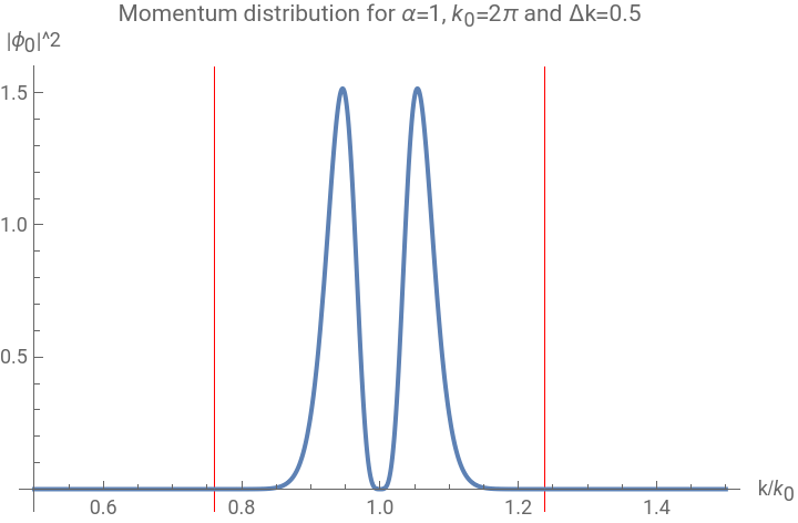
Plot the momentum distribution:
In[]:=
With[{var={k0->2π,α->1,Δk->.5}},Plot[(ϕ0//.k->k0kk/.var)^2,{kk,0.5,1.5},PlotRange->All,AxesLabel->{"k/","||^2"},GridLines->{{1+3Δk/k0/.var,1-3Δk/k0/.var},None},GridLinesStyleDirective[Red,Thin],PlotLabel->"Momentum distribution for α=1, =2π and Δk=0.5"]]
k
0
ϕ
0
k
0
Out[]=
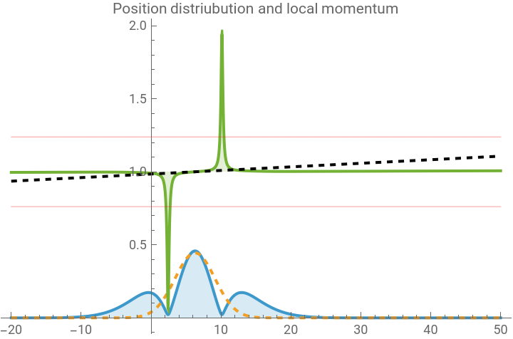
Plot the position distribution and the normalized local momentum:
In[]:=
With{var={k0->2π,α->1,Δk->.5},var0={k0->2π,α->0,Δk->.5}},ManipulatePlotAbs[ψ[x,t]/.var],Abs[ψ[x,t]/.var0],ImgradArg[x,t]/.var,1+3Δkk0/.var,1-3Δkk0/.var,ImgradArg[x,t]/.var0,{x,-20,50},PlotRange->All,Filling->{1->0,3->1},PlotLegends->{"|ψ","|","local phase momemtum/","bandwidth of momentum distribution",None,"local phase momemtum/ when α=0"},PlotStyle->{Automatic,Dashed,Automatic,Directive[Red,Thin],Directive[Red,Thin],Directive[Black,Dashed]},PlotLabel->"Position distriubution and local momentum",{t,Range[4],SetterBar},SaveDefinitions->True
1
k0
1
k0
2
|
ψ
α=0
2
|
k
0
k
0
Out[]=



In[]:=
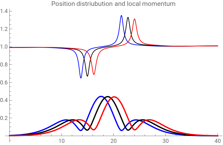
With{var={k0->2π,α->1,Δk->.5},t1=2.8,t2=3,t3=3.2},PlotAbs[ψ[x,t1]/.var],Abs[ψ[x,t2]/.var],Abs[ψ[x,t3]/.var],ImgradArg[x,t1]/.var,ImgradArg[x,t2]/.var,ImgradArg[x,t3]/.var,{x,0,40},PlotRange->All,PlotStyle->{Blue,Black,Red,Directive[Blue,Thickness[.003]],Directive[Black,Thickness[.003]],Directive[Red,Thickness[.003]]},PlotLegends->{"|","|","|","local phase momemtum/ at t=2.8","local phase momemtum/ at t=3.0","local phase momemtum/ at t=3.2"},PlotLabel->"Position distriubution and local momentum"
1
k0
1
k0
1
k0
ψ
t=2.8
2
|
ψ
t=3.0
2
|
ψ
t=3.2
2
|
k
0
k
0
k
0
Out[]=


In[]:=
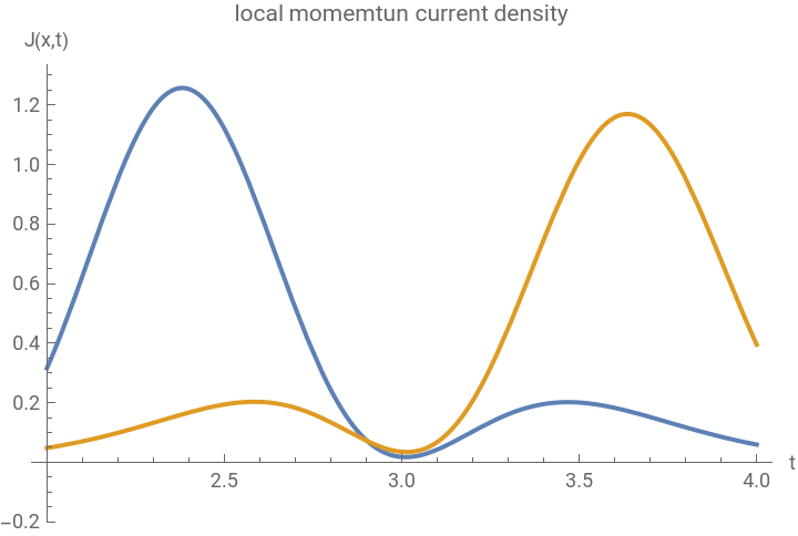
With[{var={k0->2π,α->1,Δk->.5},xPL=15.0,xPR=22.9},Plot[{Abs[ψ[xPL,t]]^2Im[gradArg[xPL,t]]/.var,Abs[ψ[xPR,t]]^2Im[gradArg[xPR,t]]/.var},{t,2,4},PlotRange->{-.2,All},PlotLabel->"local momemtun current density",AxesLabel->{"t","J(x,t)"},PlotLegends->{"J(15.0,t)","J(22.9,t)"}]]
Out[]=


Madelung trajectories
Madelung trajectories
In[]:=
pnds=ParametricNDSolveValue[{x'[t]==Im[gradArg[x[t],t]],x[0]==x0},x,{t,0,f},{x0,f,k0,α,Δk}]
Visualize the position density:
Find Madelung trajectories given some initial conditions and parameters:
Visualize them:
Plot the momentum distribution:
Plot the position distribution and the normalized local momentum:
Madelung trajectories
Madelung trajectories
Visualize the position density:
Find Madelung trajectories given some initial conditions and parameters:
Visualize them:
CITE THIS NOTEBOOK
CITE THIS NOTEBOOK
Quantum tale of the hare and tortoise
by Mohammad Bahrami
Wolfram Community, STAFF PICKS, January 17, 2025
https://community.wolfram.com/groups/-/m/t/3358663
by Mohammad Bahrami
Wolfram Community, STAFF PICKS, January 17, 2025
https://community.wolfram.com/groups/-/m/t/3358663